Loading packages
pacman::p_load(olsrr, corrplot, ggpubr,
sf,spdep, GWmodel, tmap,
tidyverse, gtsummary,patchwork, ggthemes)In previous sections we have seen how to
handle geospatial and aspatial data
plot choropleth math
compute various types of spatial weights and weight matrix
determine hotspot and coldspot areas
measure global and local measures of spatial autocorrelation
delineate homogeneous region using spatially constrained techniques
The objective of this study is to Calibrate Hedonic Pricing Model for Private Highrise Property in Singapore using Geographically Weighted Regression (GWR) Method
What is Geographically Weighted Regression?
It is a spatial statistical technique that takes non-stationary variables into consideration (e.g., climate; demographic factors; physical environment characteristics) and models the local relationships between these independent variables and an outcome of interest (also known as dependent variable).
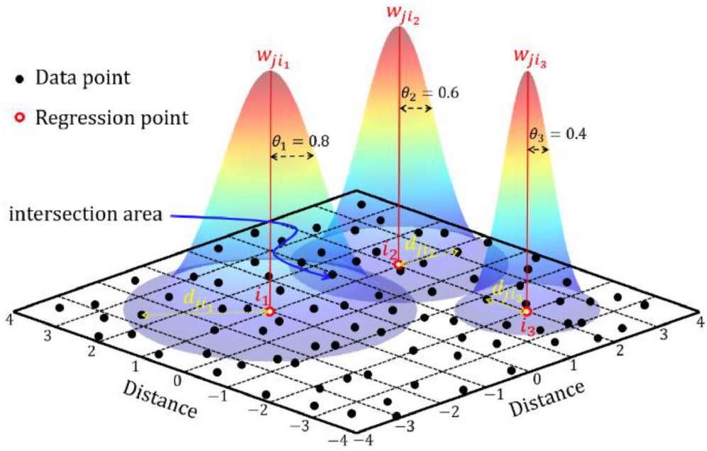
Some of the important steps performed in this study are as follows
importing geospatial data using appropriate function(s) of sf package,
importing csv file using appropriate function of readr package,
converting aspatial dataframe into sf object
performing exploratory data analysis
performing simple and multiple linear regression techniques
building a hedonic price model using GWR method
Following two data sets are used:
URA Master Plan subzone boundary in shapefile format (i.e. MP14_SUBZONE_WEB_PL)
condo_resale_2015 in csv format (i.e. condo_resale_2015.csv)
p_load function pf pacman package is used to install and load sf all necessary packages into R environment.
sf, rgdal and spdep - Spatial data handling
tidyverse, especially readr, ggplot2 and dplyr - Attribute data handling
tmap -Choropleth mapping
olsrr - Ordinary Least Square(OLS) method and performing diagnostics tests
GWmodel - geographical weighted family of models
corrplot - multivariate data visualisation and analysis
The code chunk below installs and launches these R packages into R environment.
The code chunk below is used to import MP_SUBZONE_WEB_PL shapefile by using st_read() of sf packages.
Reading layer `MP14_SUBZONE_WEB_PL' from data source
`D:\raveenaclr\Geospatial Analytics\Hands-on_Ex\data\geospatial'
using driver `ESRI Shapefile'
Simple feature collection with 323 features and 15 fields
Geometry type: MULTIPOLYGON
Dimension: XY
Bounding box: xmin: 2667.538 ymin: 15748.72 xmax: 56396.44 ymax: 50256.33
Projected CRS: SVY21The code chunk below updates the newly imported mpsz with the correct ESPG code (i.e. 3414)
Currently, the condo_resale tibble data frame is aspatial. We will convert it to a sf object. The code chunk below converts condo_resale data frame into a simple feature data frame by using st_as_sf() of sf packages.
What is the distribution of Condo selling price?
The figure above reveals a right skewed distribution. This means that more condominium units were transacted at relative lower prices. Tghis can be normalised by using log transformation.
The code chunk below is used to derive a new variable called LOG_SELLING_PRICE by using a log transformation on the variable SELLING_PRICE. It is performed using mutate() of dplyr package.
condo_resale.sf <- condo_resale.sf %>%
mutate(`LOG_SELLING_PRICE` = log(SELLING_PRICE))
h2 <- ggplot(data=condo_resale.sf,
aes(x=`LOG_SELLING_PRICE`,
y= ..density..)) +
geom_histogram(bins=20,
color="black",
fill="coral")+
geom_density(color="black",
alpha=0.5)+
theme(panel.background= element_blank())Let us compare the distribution before and after performing log transformation
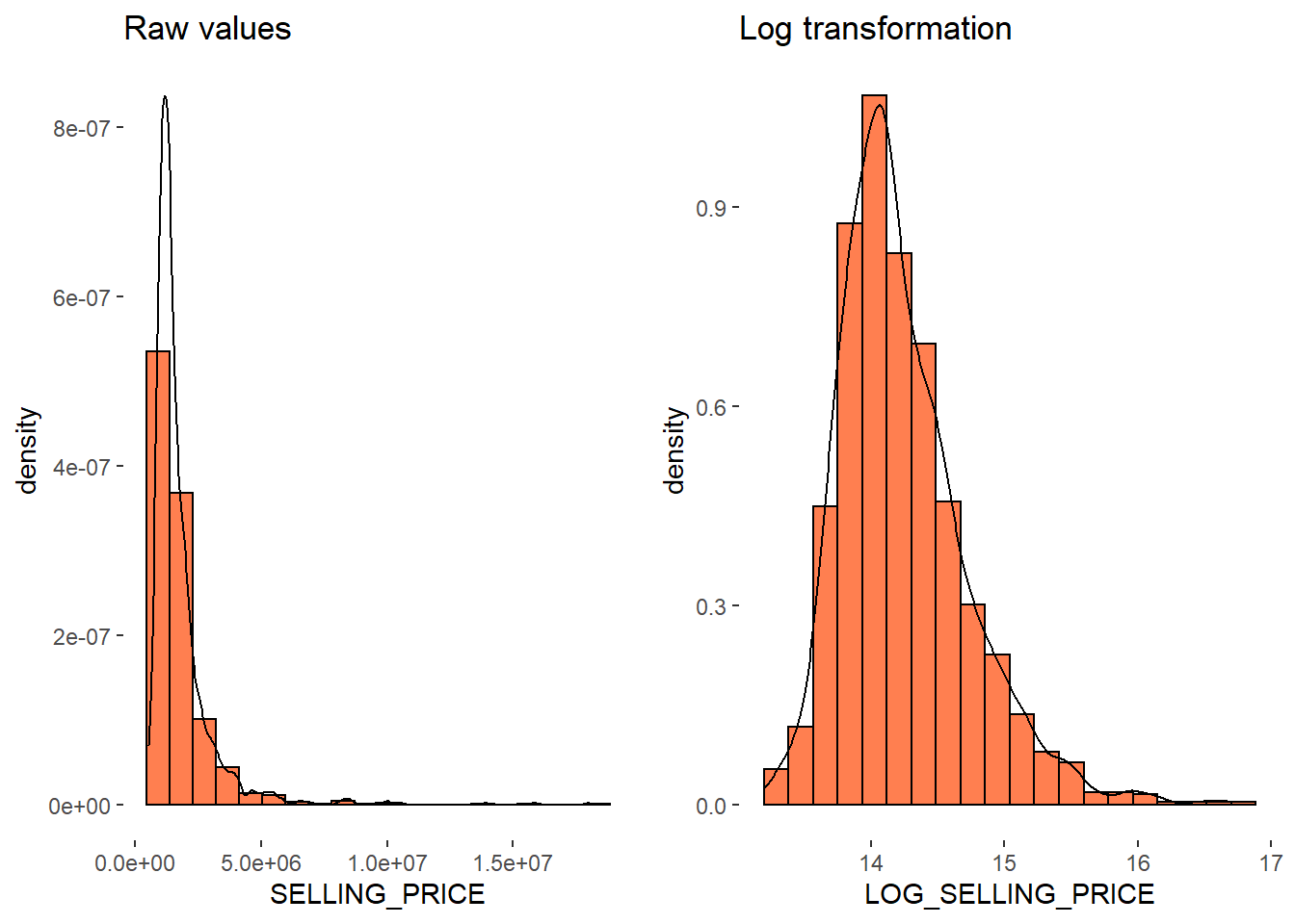
Now let us view the distribution for multiple variables
The code chunk below is used to multiple histograms. Then, ggarrange() is used to organised these histogram into a 3 columns by 4 rows small multiple plot.
AREA_SQM <- ggplot(data=condo_resale.sf,
aes(x= `AREA_SQM`,
y= ..density..)) +
geom_histogram(bins=20,
color="black",
fill="coral")+
geom_density(color="black",
alpha=0.5)+
theme(panel.background= element_blank())
AGE <- ggplot(data=condo_resale.sf,
aes(x= `AGE`,
y= ..density..)) +
geom_histogram(bins=20,
color="black",
fill="coral")+
geom_density(color="black",
alpha=0.5)+
theme(panel.background= element_blank())
PROX_CBD <- ggplot(data=condo_resale.sf,
aes(x= `PROX_CBD`,
y= ..density..)) +
geom_histogram(bins=20,
color="black",
fill="coral")+
geom_density(color="black",
alpha=0.5)+
theme(panel.background= element_blank())
PROX_CHILDCARE <- ggplot(data=condo_resale.sf,
aes(x= `PROX_CHILDCARE`,
y= ..density..)) +
geom_histogram(bins=20,
color="black",
fill="coral")+
geom_density(color="black",
alpha=0.5)+
theme(panel.background= element_blank())
PROX_ELDERLYCARE <- ggplot(data=condo_resale.sf,
aes(x= `PROX_ELDERLYCARE`,
y= ..density..)) +
geom_histogram(bins=20,
color="black",
fill="coral")+
geom_density(color="black",
alpha=0.5)+
theme(panel.background= element_blank())
PROX_URA_GROWTH_AREA <- ggplot(data=condo_resale.sf,
aes(x= `PROX_URA_GROWTH_AREA`,
y= ..density..)) +
geom_histogram(bins=20,
color="black",
fill="coral")+
geom_density(color="black",
alpha=0.5)+
theme(panel.background= element_blank())
PROX_HAWKER_MARKET <- ggplot(data=condo_resale.sf,
aes(x= `PROX_HAWKER_MARKET`,
y= ..density..)) +
geom_histogram(bins=20,
color="black",
fill="coral")+
geom_density(color="black",
alpha=0.5)+
theme(panel.background= element_blank())
PROX_KINDERGARTEN <- ggplot(data=condo_resale.sf,
aes(x= `PROX_KINDERGARTEN`,
y= ..density..)) +
geom_histogram(bins=20,
color="black",
fill="coral")+
geom_density(color="black",
alpha=0.5)+
theme(panel.background= element_blank())
PROX_MRT <- ggplot(data=condo_resale.sf,
aes(x= `PROX_MRT`,
y= ..density..)) +
geom_histogram(bins=20,
color="black",
fill="coral")+
geom_density(color="black",
alpha=0.5)+
theme(panel.background= element_blank())
PROX_PARK <- ggplot(data=condo_resale.sf,
aes(x= `PROX_PARK`,
y= ..density..)) +
geom_histogram(bins=20,
color="black",
fill="coral")+
geom_density(color="black",
alpha=0.5)+
theme(panel.background= element_blank())
PROX_PRIMARY_SCH <- ggplot(data=condo_resale.sf,
aes(x= `PROX_PRIMARY_SCH`,
y= ..density..)) +
geom_histogram(bins=20,
color="black",
fill="coral")+
geom_density(color="black",
alpha=0.5)+
theme(panel.background= element_blank())
PROX_TOP_PRIMARY_SCH <- ggplot(data=condo_resale.sf,
aes(x= `PROX_TOP_PRIMARY_SCH`,
y= ..density..)) +
geom_histogram(bins=20,
color="black",
fill="coral")+
geom_density(color="black",
alpha=0.5)+
theme(panel.background= element_blank())
ggarrange(AREA_SQM, AGE, PROX_CBD, PROX_CHILDCARE, PROX_ELDERLYCARE,
PROX_URA_GROWTH_AREA, PROX_HAWKER_MARKET, PROX_KINDERGARTEN, PROX_MRT,
PROX_PARK, PROX_PRIMARY_SCH, PROX_TOP_PRIMARY_SCH,
ncol = 3, nrow = 4)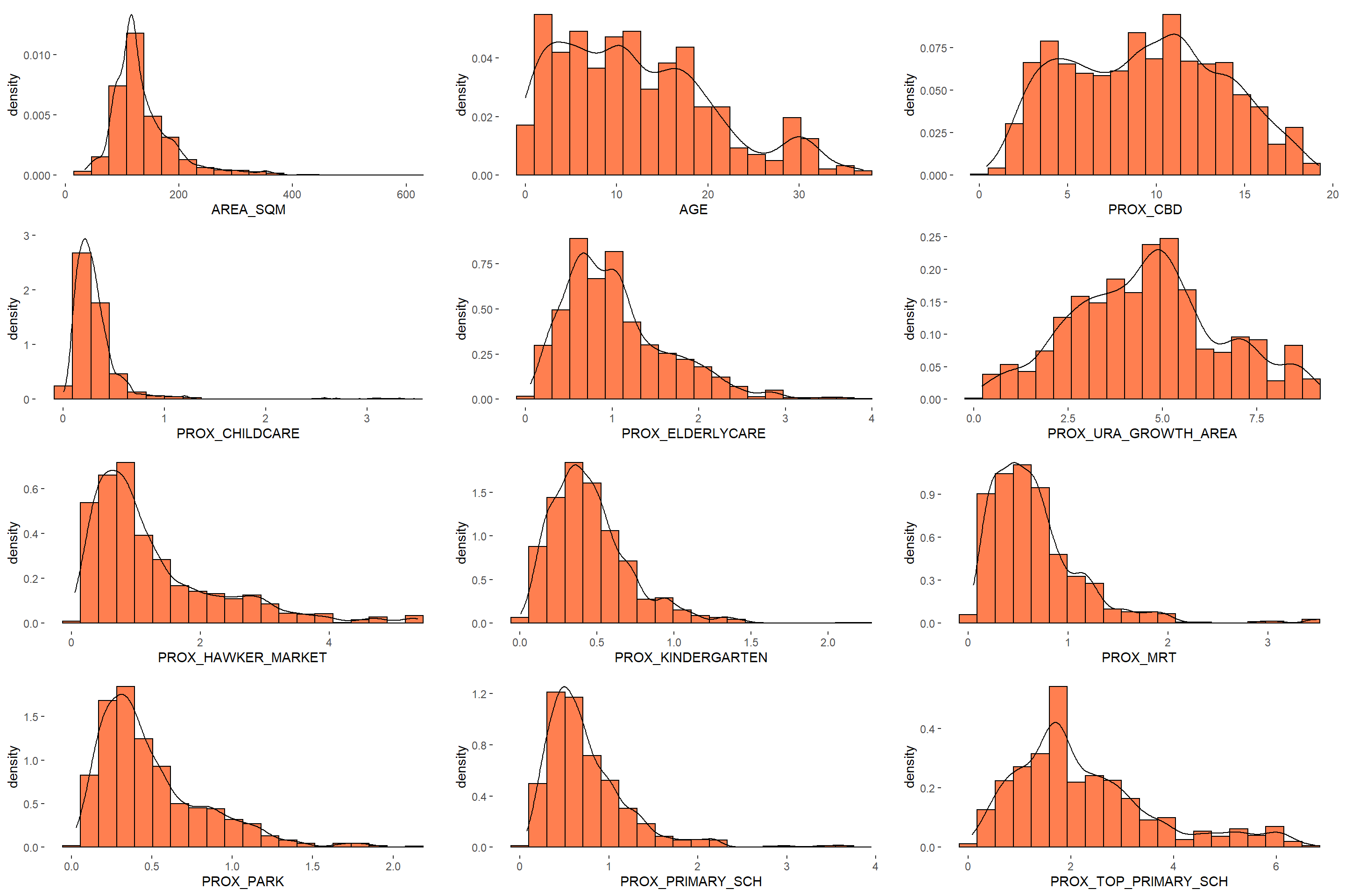
What is the geospatial distribution of condo prices in Singapore?
The code chunks below is used to create an interactive point symbol map.
tmap mode set to interactive viewingWarning: The shape mpsz_svy21 is invalid (after reprojection). See
sf::st_is_validFirst, let us build a simple linear regression model by using SELLING_PRICE as the dependent variable and AREA_SQM as the independent variable.
Call:
lm(formula = SELLING_PRICE ~ AREA_SQM, data = condo_resale.sf)
Residuals:
Min 1Q Median 3Q Max
-3695815 -391764 -87517 258900 13503875
Coefficients:
Estimate Std. Error t value Pr(>|t|)
(Intercept) -258121.1 63517.2 -4.064 5.09e-05 ***
AREA_SQM 14719.0 428.1 34.381 < 2e-16 ***
---
Signif. codes: 0 '***' 0.001 '**' 0.01 '*' 0.05 '.' 0.1 ' ' 1
Residual standard error: 942700 on 1434 degrees of freedom
Multiple R-squared: 0.4518, Adjusted R-squared: 0.4515
F-statistic: 1182 on 1 and 1434 DF, p-value: < 2.2e-16Interpretation
R-squared of 0.4518 reveals that the simple regression model built is able to explain about 45% of the resale prices.
H0 (Null Hypothesis) - mean price is a good estimator of SELLING_PRICE
H1 (Alternative Hypothesis) - mean price is not a good estimator of SELLING_PRICE
Since p-value is much smaller than 0.0001, we will reject the null hypothesis that mean is a good estimator of SELLING_PRICE.
This will allow us to infer that simple linear regression model above is a good estimator of SELLING_PRICE.
p-values of both the estimates of the Intercept and ARA_SQM are smaller than 0.001. In view of this, the null hypothesis of the B0 and B1 are equal to 0 will be rejected and so B0 and B1 are good parameter estimates.
Let us visualise the best fit curve on a scatterplot, using lm() as a method function in ggplot’s geometry as shown in the code chunk below.
`geom_smooth()` using formula 'y ~ x'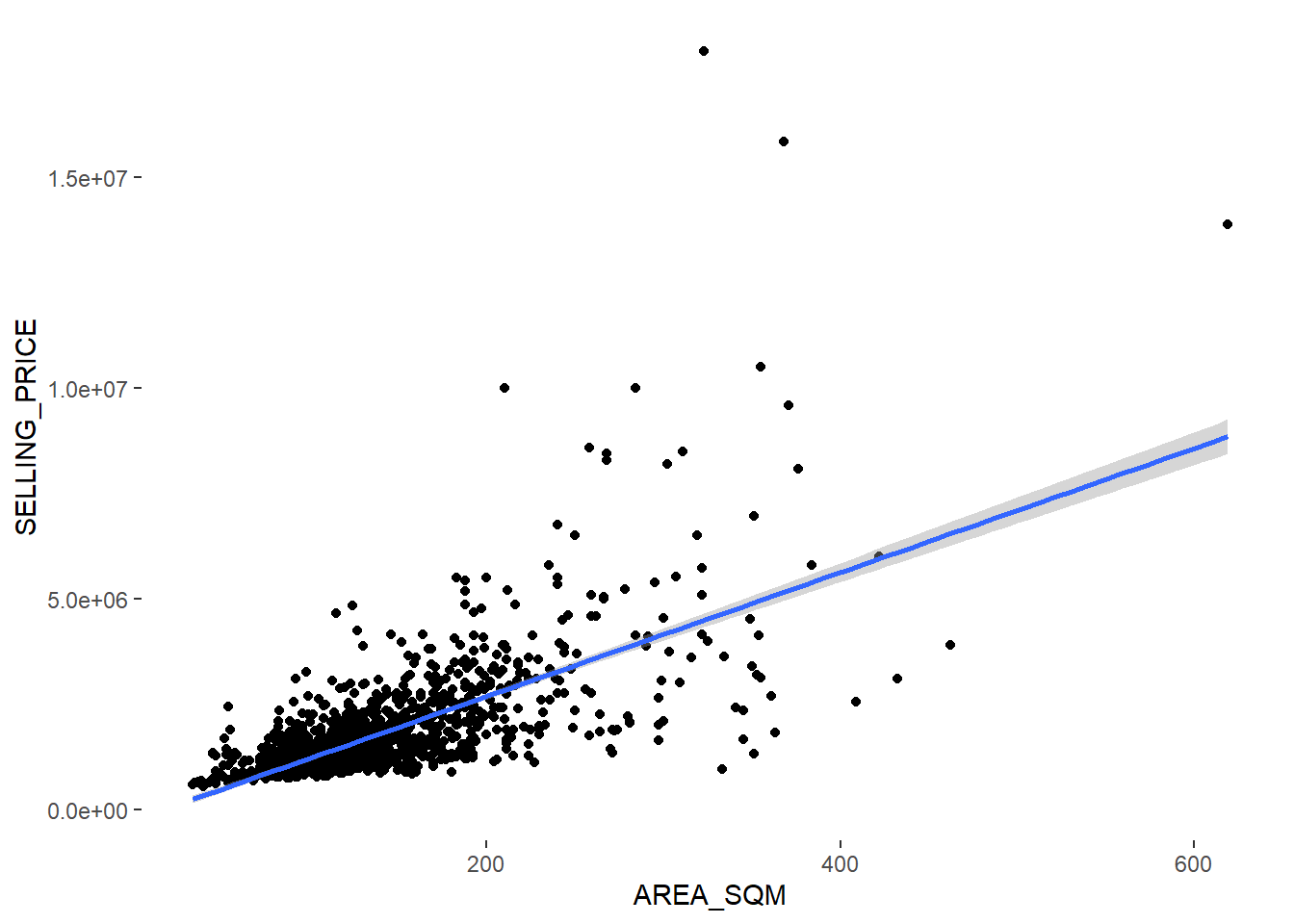
We can see that there are a few statistical outliers with relatively high selling prices.
Let us check if there is a multicollinearity phenomenon by executing correlation analysis. It is important to ensure that the indepdent variables used are not highly correlated to each other.
The code chunk below is used to plot a scatterplot matrix of the relationship between the independent variables in condo_resale data.frame.
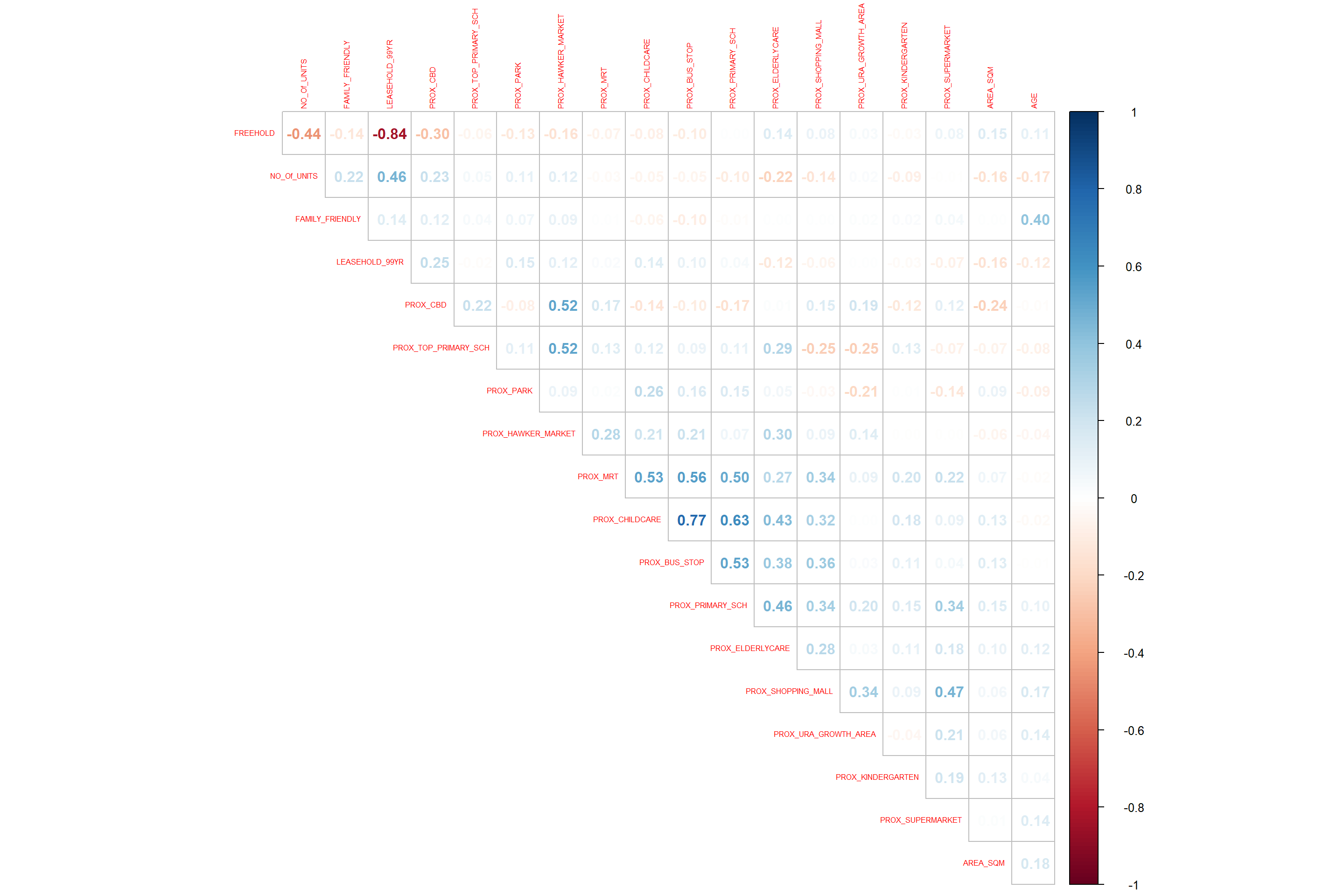
It is clear that Freehold is highly correlated to LEASE_99YEAR. Hence, let us include either one of them i.e. LEASE_99YEAR in the subsequent model building.
The code chunk below using lm() to calibrate the multiple linear regression model.
condo.mlr <- lm(formula = SELLING_PRICE ~ AREA_SQM + AGE +
PROX_CBD + PROX_CHILDCARE + PROX_ELDERLYCARE +
PROX_URA_GROWTH_AREA + PROX_HAWKER_MARKET + PROX_KINDERGARTEN +
PROX_MRT + PROX_PARK + PROX_PRIMARY_SCH +
PROX_TOP_PRIMARY_SCH + PROX_SHOPPING_MALL + PROX_SUPERMARKET +
PROX_BUS_STOP + NO_Of_UNITS + FAMILY_FRIENDLY + FREEHOLD,
data=condo_resale.sf)
summary(condo.mlr)
Call:
lm(formula = SELLING_PRICE ~ AREA_SQM + AGE + PROX_CBD + PROX_CHILDCARE +
PROX_ELDERLYCARE + PROX_URA_GROWTH_AREA + PROX_HAWKER_MARKET +
PROX_KINDERGARTEN + PROX_MRT + PROX_PARK + PROX_PRIMARY_SCH +
PROX_TOP_PRIMARY_SCH + PROX_SHOPPING_MALL + PROX_SUPERMARKET +
PROX_BUS_STOP + NO_Of_UNITS + FAMILY_FRIENDLY + FREEHOLD,
data = condo_resale.sf)
Residuals:
Min 1Q Median 3Q Max
-3475964 -293923 -23069 241043 12260381
Coefficients:
Estimate Std. Error t value Pr(>|t|)
(Intercept) 481728.40 121441.01 3.967 7.65e-05 ***
AREA_SQM 12708.32 369.59 34.385 < 2e-16 ***
AGE -24440.82 2763.16 -8.845 < 2e-16 ***
PROX_CBD -78669.78 6768.97 -11.622 < 2e-16 ***
PROX_CHILDCARE -351617.91 109467.25 -3.212 0.00135 **
PROX_ELDERLYCARE 171029.42 42110.51 4.061 5.14e-05 ***
PROX_URA_GROWTH_AREA 38474.53 12523.57 3.072 0.00217 **
PROX_HAWKER_MARKET 23746.10 29299.76 0.810 0.41782
PROX_KINDERGARTEN 147468.99 82668.87 1.784 0.07466 .
PROX_MRT -314599.68 57947.44 -5.429 6.66e-08 ***
PROX_PARK 563280.50 66551.68 8.464 < 2e-16 ***
PROX_PRIMARY_SCH 180186.08 65237.95 2.762 0.00582 **
PROX_TOP_PRIMARY_SCH 2280.04 20410.43 0.112 0.91107
PROX_SHOPPING_MALL -206604.06 42840.60 -4.823 1.57e-06 ***
PROX_SUPERMARKET -44991.80 77082.64 -0.584 0.55953
PROX_BUS_STOP 683121.35 138353.28 4.938 8.85e-07 ***
NO_Of_UNITS -231.18 89.03 -2.597 0.00951 **
FAMILY_FRIENDLY 140340.77 47020.55 2.985 0.00289 **
FREEHOLD 359913.01 49220.22 7.312 4.38e-13 ***
---
Signif. codes: 0 '***' 0.001 '**' 0.01 '*' 0.05 '.' 0.1 ' ' 1
Residual standard error: 755800 on 1417 degrees of freedom
Multiple R-squared: 0.6518, Adjusted R-squared: 0.6474
F-statistic: 147.4 on 18 and 1417 DF, p-value: < 2.2e-16At 99% confidence interval, almost all the varibles are statistically significant except PROX_HAWKER_MARKET, PROX_KINDERGARTEN , PROX_TOP_PRIMARY_SCH.
It is clear that not all the independent variables are statistically significant. Let us revise the model by removing those variables which are not statistically significant.
Model Summary
------------------------------------------------------------------------
R 0.807 RMSE 755957.289
R-Squared 0.651 Coef. Var 43.168
Adj. R-Squared 0.647 MSE 571471422208.591
Pred R-Squared 0.638 MAE 414819.628
------------------------------------------------------------------------
RMSE: Root Mean Square Error
MSE: Mean Square Error
MAE: Mean Absolute Error
ANOVA
--------------------------------------------------------------------------------
Sum of
Squares DF Mean Square F Sig.
--------------------------------------------------------------------------------
Regression 1.512586e+15 14 1.080418e+14 189.059 0.0000
Residual 8.120609e+14 1421 571471422208.591
Total 2.324647e+15 1435
--------------------------------------------------------------------------------
Parameter Estimates
-----------------------------------------------------------------------------------------------------------------
model Beta Std. Error Std. Beta t Sig lower upper
-----------------------------------------------------------------------------------------------------------------
(Intercept) 527633.222 108183.223 4.877 0.000 315417.244 739849.200
AREA_SQM 12777.523 367.479 0.584 34.771 0.000 12056.663 13498.382
AGE -24687.739 2754.845 -0.167 -8.962 0.000 -30091.739 -19283.740
PROX_CBD -77131.323 5763.125 -0.263 -13.384 0.000 -88436.469 -65826.176
PROX_CHILDCARE -318472.751 107959.512 -0.084 -2.950 0.003 -530249.889 -106695.613
PROX_ELDERLYCARE 185575.623 39901.864 0.090 4.651 0.000 107302.737 263848.510
PROX_URA_GROWTH_AREA 39163.254 11754.829 0.060 3.332 0.001 16104.571 62221.936
PROX_MRT -294745.107 56916.367 -0.112 -5.179 0.000 -406394.234 -183095.980
PROX_PARK 570504.807 65507.029 0.150 8.709 0.000 442003.938 699005.677
PROX_PRIMARY_SCH 159856.136 60234.599 0.062 2.654 0.008 41697.849 278014.424
PROX_SHOPPING_MALL -220947.251 36561.832 -0.115 -6.043 0.000 -292668.213 -149226.288
PROX_BUS_STOP 682482.221 134513.243 0.134 5.074 0.000 418616.359 946348.082
NO_Of_UNITS -245.480 87.947 -0.053 -2.791 0.005 -418.000 -72.961
FAMILY_FRIENDLY 146307.576 46893.021 0.057 3.120 0.002 54320.593 238294.560
FREEHOLD 350599.812 48506.485 0.136 7.228 0.000 255447.802 445751.821
-----------------------------------------------------------------------------------------------------------------Now, we have only statistically significant variables.
In the code chunk below, tbl_regression() is used to create a well formatted regression report using gtsummary package that provides an elegant and flexible way to create publication-ready summary tables in R.
| Characteristic | Beta | 95% CI1 | p-value |
|---|---|---|---|
| (Intercept) | 527,633 | 315,417, 739,849 | <0.001 |
| AREA_SQM | 12,778 | 12,057, 13,498 | <0.001 |
| AGE | -24,688 | -30,092, -19,284 | <0.001 |
| PROX_CBD | -77,131 | -88,436, -65,826 | <0.001 |
| PROX_CHILDCARE | -318,473 | -530,250, -106,696 | 0.003 |
| PROX_ELDERLYCARE | 185,576 | 107,303, 263,849 | <0.001 |
| PROX_URA_GROWTH_AREA | 39,163 | 16,105, 62,222 | <0.001 |
| PROX_MRT | -294,745 | -406,394, -183,096 | <0.001 |
| PROX_PARK | 570,505 | 442,004, 699,006 | <0.001 |
| PROX_PRIMARY_SCH | 159,856 | 41,698, 278,014 | 0.008 |
| PROX_SHOPPING_MALL | -220,947 | -292,668, -149,226 | <0.001 |
| PROX_BUS_STOP | 682,482 | 418,616, 946,348 | <0.001 |
| NO_Of_UNITS | -245 | -418, -73 | 0.005 |
| FAMILY_FRIENDLY | 146,308 | 54,321, 238,295 | 0.002 |
| FREEHOLD | 350,600 | 255,448, 445,752 | <0.001 |
| 1 CI = Confidence Interval | |||
With this, model statistics can also be included in the report by either appending them to the report table by using add_glance_table() or adding as a table source note by using add_glance_source_note() as shown in the code chunk below.
| Characteristic | Beta | 95% CI1 | p-value |
|---|---|---|---|
| (Intercept) | 527,633 | 315,417, 739,849 | <0.001 |
| AREA_SQM | 12,778 | 12,057, 13,498 | <0.001 |
| AGE | -24,688 | -30,092, -19,284 | <0.001 |
| PROX_CBD | -77,131 | -88,436, -65,826 | <0.001 |
| PROX_CHILDCARE | -318,473 | -530,250, -106,696 | 0.003 |
| PROX_ELDERLYCARE | 185,576 | 107,303, 263,849 | <0.001 |
| PROX_URA_GROWTH_AREA | 39,163 | 16,105, 62,222 | <0.001 |
| PROX_MRT | -294,745 | -406,394, -183,096 | <0.001 |
| PROX_PARK | 570,505 | 442,004, 699,006 | <0.001 |
| PROX_PRIMARY_SCH | 159,856 | 41,698, 278,014 | 0.008 |
| PROX_SHOPPING_MALL | -220,947 | -292,668, -149,226 | <0.001 |
| PROX_BUS_STOP | 682,482 | 418,616, 946,348 | <0.001 |
| NO_Of_UNITS | -245 | -418, -73 | 0.005 |
| FAMILY_FRIENDLY | 146,308 | 54,321, 238,295 | 0.002 |
| FREEHOLD | 350,600 | 255,448, 445,752 | <0.001 |
| R² = 0.651; Adjusted R² = 0.647; AIC = 42,967; Statistic = 189; p-value = <0.001; σ = 755,957 | |||
| 1 CI = Confidence Interval | |||
Let us check if there is any sign of multicollinearity using ols_vif_tol() of olsrr package
Variables Tolerance VIF
1 AREA_SQM 0.8728554 1.145665
2 AGE 0.7071275 1.414172
3 PROX_CBD 0.6356147 1.573280
4 PROX_CHILDCARE 0.3066019 3.261559
5 PROX_ELDERLYCARE 0.6598479 1.515501
6 PROX_URA_GROWTH_AREA 0.7510311 1.331503
7 PROX_MRT 0.5236090 1.909822
8 PROX_PARK 0.8279261 1.207837
9 PROX_PRIMARY_SCH 0.4524628 2.210126
10 PROX_SHOPPING_MALL 0.6738795 1.483945
11 PROX_BUS_STOP 0.3514118 2.845664
12 NO_Of_UNITS 0.6901036 1.449058
13 FAMILY_FRIENDLY 0.7244157 1.380423
14 FREEHOLD 0.6931163 1.442759We can conclude that there are no sign of multicollinearity among the independent variables as VIF of the independent variables are less than 10.
In the code chunk below, the ols_plot_resid_fit() of olsrr package is used to perform linearity assumption test.
We can conclude that the relationships between the dependent variable and independent variables are linear as most of the data poitns are scattered around the 0 line.
The code chunk below uses ols_plot_resid_hist() of olsrr package to perform normality assumption test.
It is shown that the residual of the multiple linear regression model (i.e. condo.mlr1) resembles normal distribution.
In order to perform spatial autocorrelation test, let us perform the following steps
Convert condo_resale.sf from sf data frame into a SpatialPointsDataFrame.
Convert condo_resale.res.sf from simple feature object into a SpatialPointsDataFrame because spdep package can only process sp conformed spatial data objects.
Display the distribution of the residuals on an interactive map
Let us visualise the spatial distribution using below code chunk
tmap mode set to interactive viewingWarning: The shape mpsz_svy21 is invalid (after reprojection). See
sf::st_is_validVariable(s) "MLR_RES" contains positive and negative values, so midpoint is set to 0. Set midpoint = NA to show the full spectrum of the color palette.The figure above reveal that there is sign of spatial autocorrelation.
Let us double check by performing Moran’s I test
Following steps will be performed
Compute the distance-based weight matrix by using dnearneigh() function of spdep.
Convert the output neighbours lists (i.e. nb) into a spatial weights using nb2listw() of spdep packge.
Conduct Moran’s I test for residual spatial autocorrelation by using lm.morantest() of spdep package.
Global Moran I for regression residuals
data:
model: lm(formula = SELLING_PRICE ~ AREA_SQM + AGE + PROX_CBD +
PROX_CHILDCARE + PROX_ELDERLYCARE + PROX_URA_GROWTH_AREA + PROX_MRT +
PROX_PARK + PROX_PRIMARY_SCH + PROX_SHOPPING_MALL + PROX_BUS_STOP +
NO_Of_UNITS + FAMILY_FRIENDLY + FREEHOLD, data = condo_resale.sf)
weights: nb_lw
Moran I statistic standard deviate = 24.366, p-value < 2.2e-16
alternative hypothesis: greater
sample estimates:
Observed Moran I Expectation Variance
1.438876e-01 -5.487594e-03 3.758259e-05 Since the Observed Global Moran I = 0.1424418 which is greater than 0, we can infer than the residuals resemble cluster distribution.
Let us model hedonic pricing using both the fixed and adaptive bandwidth schemes
In the code chunk below bw.gwr() of GWModel package is used to determine the optimal fixed bandwidth to use in the model.
bw.fixed <- bw.gwr(formula = SELLING_PRICE ~ AREA_SQM + AGE + PROX_CBD +
PROX_CHILDCARE + PROX_ELDERLYCARE + PROX_URA_GROWTH_AREA +
PROX_MRT + PROX_PARK + PROX_PRIMARY_SCH +
PROX_SHOPPING_MALL + PROX_BUS_STOP + NO_Of_UNITS +
FAMILY_FRIENDLY + FREEHOLD,
data=condo_resale.sp,
approach="CV",
kernel="gaussian",
adaptive=FALSE,
longlat=FALSE)Fixed bandwidth: 17660.96 CV score: 8.259118e+14
Fixed bandwidth: 10917.26 CV score: 7.970454e+14
Fixed bandwidth: 6749.419 CV score: 7.273273e+14
Fixed bandwidth: 4173.553 CV score: 6.300006e+14
Fixed bandwidth: 2581.58 CV score: 5.404958e+14
Fixed bandwidth: 1597.687 CV score: 4.857515e+14
Fixed bandwidth: 989.6077 CV score: 4.722431e+14
Fixed bandwidth: 613.7939 CV score: 1.378294e+16
Fixed bandwidth: 1221.873 CV score: 4.778717e+14
Fixed bandwidth: 846.0596 CV score: 4.791629e+14
Fixed bandwidth: 1078.325 CV score: 4.751406e+14
Fixed bandwidth: 934.7772 CV score: 4.72518e+14
Fixed bandwidth: 1023.495 CV score: 4.730305e+14
Fixed bandwidth: 968.6643 CV score: 4.721317e+14
Fixed bandwidth: 955.7206 CV score: 4.722072e+14
Fixed bandwidth: 976.6639 CV score: 4.721387e+14
Fixed bandwidth: 963.7202 CV score: 4.721484e+14
Fixed bandwidth: 971.7199 CV score: 4.721293e+14
Fixed bandwidth: 973.6083 CV score: 4.721309e+14
Fixed bandwidth: 970.5527 CV score: 4.721295e+14
Fixed bandwidth: 972.4412 CV score: 4.721296e+14
Fixed bandwidth: 971.2741 CV score: 4.721292e+14
Fixed bandwidth: 970.9985 CV score: 4.721293e+14
Fixed bandwidth: 971.4443 CV score: 4.721292e+14
Fixed bandwidth: 971.5496 CV score: 4.721293e+14
Fixed bandwidth: 971.3793 CV score: 4.721292e+14
Fixed bandwidth: 971.3391 CV score: 4.721292e+14
Fixed bandwidth: 971.3143 CV score: 4.721292e+14
Fixed bandwidth: 971.3545 CV score: 4.721292e+14
Fixed bandwidth: 971.3296 CV score: 4.721292e+14
Fixed bandwidth: 971.345 CV score: 4.721292e+14
Fixed bandwidth: 971.3355 CV score: 4.721292e+14
Fixed bandwidth: 971.3413 CV score: 4.721292e+14
Fixed bandwidth: 971.3377 CV score: 4.721292e+14
Fixed bandwidth: 971.34 CV score: 4.721292e+14
Fixed bandwidth: 971.3405 CV score: 4.721292e+14
Fixed bandwidth: 971.3408 CV score: 4.721292e+14
Fixed bandwidth: 971.3403 CV score: 4.721292e+14
Fixed bandwidth: 971.3406 CV score: 4.721292e+14
Fixed bandwidth: 971.3404 CV score: 4.721292e+14
Fixed bandwidth: 971.3405 CV score: 4.721292e+14
Fixed bandwidth: 971.3405 CV score: 4.721292e+14 The result shows that the recommended bandwidth is 971.3398 metres
Let us calibrate the gwr model using fixed bandwidth and gaussian kernel.
gwr.fixed <- gwr.basic(formula = SELLING_PRICE ~ AREA_SQM + AGE + PROX_CBD +
PROX_CHILDCARE + PROX_ELDERLYCARE + PROX_URA_GROWTH_AREA +
PROX_MRT + PROX_PARK + PROX_PRIMARY_SCH +
PROX_SHOPPING_MALL + PROX_BUS_STOP + NO_Of_UNITS +
FAMILY_FRIENDLY + FREEHOLD,
data=condo_resale.sp,
bw=bw.fixed,
kernel = 'gaussian',
longlat = FALSE) ***********************************************************************
* Package GWmodel *
***********************************************************************
Program starts at: 2022-12-19 07:45:04
Call:
gwr.basic(formula = SELLING_PRICE ~ AREA_SQM + AGE + PROX_CBD +
PROX_CHILDCARE + PROX_ELDERLYCARE + PROX_URA_GROWTH_AREA +
PROX_MRT + PROX_PARK + PROX_PRIMARY_SCH + PROX_SHOPPING_MALL +
PROX_BUS_STOP + NO_Of_UNITS + FAMILY_FRIENDLY + FREEHOLD,
data = condo_resale.sp, bw = bw.fixed, kernel = "gaussian",
longlat = FALSE)
Dependent (y) variable: SELLING_PRICE
Independent variables: AREA_SQM AGE PROX_CBD PROX_CHILDCARE PROX_ELDERLYCARE PROX_URA_GROWTH_AREA PROX_MRT PROX_PARK PROX_PRIMARY_SCH PROX_SHOPPING_MALL PROX_BUS_STOP NO_Of_UNITS FAMILY_FRIENDLY FREEHOLD
Number of data points: 1436
***********************************************************************
* Results of Global Regression *
***********************************************************************
Call:
lm(formula = formula, data = data)
Residuals:
Min 1Q Median 3Q Max
-3470778 -298119 -23481 248917 12234210
Coefficients:
Estimate Std. Error t value Pr(>|t|)
(Intercept) 527633.22 108183.22 4.877 1.20e-06 ***
AREA_SQM 12777.52 367.48 34.771 < 2e-16 ***
AGE -24687.74 2754.84 -8.962 < 2e-16 ***
PROX_CBD -77131.32 5763.12 -13.384 < 2e-16 ***
PROX_CHILDCARE -318472.75 107959.51 -2.950 0.003231 **
PROX_ELDERLYCARE 185575.62 39901.86 4.651 3.61e-06 ***
PROX_URA_GROWTH_AREA 39163.25 11754.83 3.332 0.000885 ***
PROX_MRT -294745.11 56916.37 -5.179 2.56e-07 ***
PROX_PARK 570504.81 65507.03 8.709 < 2e-16 ***
PROX_PRIMARY_SCH 159856.14 60234.60 2.654 0.008046 **
PROX_SHOPPING_MALL -220947.25 36561.83 -6.043 1.93e-09 ***
PROX_BUS_STOP 682482.22 134513.24 5.074 4.42e-07 ***
NO_Of_UNITS -245.48 87.95 -2.791 0.005321 **
FAMILY_FRIENDLY 146307.58 46893.02 3.120 0.001845 **
FREEHOLD 350599.81 48506.48 7.228 7.98e-13 ***
---Significance stars
Signif. codes: 0 '***' 0.001 '**' 0.01 '*' 0.05 '.' 0.1 ' ' 1
Residual standard error: 756000 on 1421 degrees of freedom
Multiple R-squared: 0.6507
Adjusted R-squared: 0.6472
F-statistic: 189.1 on 14 and 1421 DF, p-value: < 2.2e-16
***Extra Diagnostic information
Residual sum of squares: 8.120609e+14
Sigma(hat): 752522.9
AIC: 42966.76
AICc: 42967.14
BIC: 41731.39
***********************************************************************
* Results of Geographically Weighted Regression *
***********************************************************************
*********************Model calibration information*********************
Kernel function: gaussian
Fixed bandwidth: 971.3405
Regression points: the same locations as observations are used.
Distance metric: Euclidean distance metric is used.
****************Summary of GWR coefficient estimates:******************
Min. 1st Qu. Median 3rd Qu.
Intercept -3.5988e+07 -5.1998e+05 7.6780e+05 1.7412e+06
AREA_SQM 1.0003e+03 5.2758e+03 7.4740e+03 1.2301e+04
AGE -1.3475e+05 -2.0813e+04 -8.6260e+03 -3.7784e+03
PROX_CBD -7.7047e+07 -2.3608e+05 -8.3600e+04 3.4646e+04
PROX_CHILDCARE -6.0097e+06 -3.3667e+05 -9.7425e+04 2.9007e+05
PROX_ELDERLYCARE -3.5000e+06 -1.5970e+05 3.1971e+04 1.9577e+05
PROX_URA_GROWTH_AREA -3.0170e+06 -8.2013e+04 7.0749e+04 2.2612e+05
PROX_MRT -3.5282e+06 -6.5836e+05 -1.8833e+05 3.6922e+04
PROX_PARK -1.2062e+06 -2.1732e+05 3.5383e+04 4.1335e+05
PROX_PRIMARY_SCH -2.2695e+07 -1.7066e+05 4.8472e+04 5.1555e+05
PROX_SHOPPING_MALL -7.2585e+06 -1.6684e+05 -1.0517e+04 1.5923e+05
PROX_BUS_STOP -1.4676e+06 -4.5207e+04 3.7601e+05 1.1664e+06
NO_Of_UNITS -1.3170e+03 -2.4822e+02 -3.0846e+01 2.5496e+02
FAMILY_FRIENDLY -2.2749e+06 -1.1140e+05 7.6214e+03 1.6107e+05
FREEHOLD -9.2067e+06 3.8073e+04 1.5169e+05 3.7528e+05
Max.
Intercept 112793548
AREA_SQM 21575
AGE 434201
PROX_CBD 2704596
PROX_CHILDCARE 1654087
PROX_ELDERLYCARE 38867814
PROX_URA_GROWTH_AREA 78515730
PROX_MRT 3124316
PROX_PARK 18122425
PROX_PRIMARY_SCH 4637503
PROX_SHOPPING_MALL 1529952
PROX_BUS_STOP 11342182
NO_Of_UNITS 12907
FAMILY_FRIENDLY 1720744
FREEHOLD 6073636
************************Diagnostic information*************************
Number of data points: 1436
Effective number of parameters (2trace(S) - trace(S'S)): 438.3804
Effective degrees of freedom (n-2trace(S) + trace(S'S)): 997.6196
AICc (GWR book, Fotheringham, et al. 2002, p. 61, eq 2.33): 42263.61
AIC (GWR book, Fotheringham, et al. 2002,GWR p. 96, eq. 4.22): 41632.36
BIC (GWR book, Fotheringham, et al. 2002,GWR p. 61, eq. 2.34): 42515.71
Residual sum of squares: 2.53407e+14
R-square value: 0.8909912
Adjusted R-square value: 0.8430417
***********************************************************************
Program stops at: 2022-12-19 07:45:06 The report shows that the adjusted r-square of the gwr is 0.8430 which is significantly better than the global multiple linear regression model of 0.6472.
Let us calibrate the gwr-absed hedonic pricing model by using adaptive bandwidth approach.
Computing the adaptive bandwidth
In the code chunk below bw.gwr() of GWModel package is used to determine the optimal fixed bandwidth with adaptive = TRUE to use in the model.
bw.adaptive <- bw.gwr(formula = SELLING_PRICE ~ AREA_SQM + AGE +
PROX_CBD + PROX_CHILDCARE + PROX_ELDERLYCARE +
PROX_URA_GROWTH_AREA + PROX_MRT + PROX_PARK +
PROX_PRIMARY_SCH + PROX_SHOPPING_MALL + PROX_BUS_STOP +
NO_Of_UNITS + FAMILY_FRIENDLY + FREEHOLD,
data=condo_resale.sp,
approach="CV",
kernel="gaussian",
adaptive=TRUE,
longlat=FALSE)Adaptive bandwidth: 895 CV score: 7.952401e+14
Adaptive bandwidth: 561 CV score: 7.667364e+14
Adaptive bandwidth: 354 CV score: 6.953454e+14
Adaptive bandwidth: 226 CV score: 6.15223e+14
Adaptive bandwidth: 147 CV score: 5.674373e+14
Adaptive bandwidth: 98 CV score: 5.426745e+14
Adaptive bandwidth: 68 CV score: 5.168117e+14
Adaptive bandwidth: 49 CV score: 4.859631e+14
Adaptive bandwidth: 37 CV score: 4.646518e+14
Adaptive bandwidth: 30 CV score: 4.422088e+14
Adaptive bandwidth: 25 CV score: 4.430816e+14
Adaptive bandwidth: 32 CV score: 4.505602e+14
Adaptive bandwidth: 27 CV score: 4.462172e+14
Adaptive bandwidth: 30 CV score: 4.422088e+14 The result reveals that 30 is the recommended data points to be used.
Let us calibrate the gwr-based hedonic pricing model by using adaptive bandwidth and gaussian kernel as shown in the code chunk below.
gwr.adaptive <- gwr.basic(formula = SELLING_PRICE ~ AREA_SQM + AGE +
PROX_CBD + PROX_CHILDCARE + PROX_ELDERLYCARE +
PROX_URA_GROWTH_AREA + PROX_MRT + PROX_PARK +
PROX_PRIMARY_SCH + PROX_SHOPPING_MALL + PROX_BUS_STOP +
NO_Of_UNITS + FAMILY_FRIENDLY + FREEHOLD,
data=condo_resale.sp, bw=bw.adaptive,
kernel = 'gaussian',
adaptive=TRUE,
longlat = FALSE)
gwr.adaptive ***********************************************************************
* Package GWmodel *
***********************************************************************
Program starts at: 2022-12-19 07:45:17
Call:
gwr.basic(formula = SELLING_PRICE ~ AREA_SQM + AGE + PROX_CBD +
PROX_CHILDCARE + PROX_ELDERLYCARE + PROX_URA_GROWTH_AREA +
PROX_MRT + PROX_PARK + PROX_PRIMARY_SCH + PROX_SHOPPING_MALL +
PROX_BUS_STOP + NO_Of_UNITS + FAMILY_FRIENDLY + FREEHOLD,
data = condo_resale.sp, bw = bw.adaptive, kernel = "gaussian",
adaptive = TRUE, longlat = FALSE)
Dependent (y) variable: SELLING_PRICE
Independent variables: AREA_SQM AGE PROX_CBD PROX_CHILDCARE PROX_ELDERLYCARE PROX_URA_GROWTH_AREA PROX_MRT PROX_PARK PROX_PRIMARY_SCH PROX_SHOPPING_MALL PROX_BUS_STOP NO_Of_UNITS FAMILY_FRIENDLY FREEHOLD
Number of data points: 1436
***********************************************************************
* Results of Global Regression *
***********************************************************************
Call:
lm(formula = formula, data = data)
Residuals:
Min 1Q Median 3Q Max
-3470778 -298119 -23481 248917 12234210
Coefficients:
Estimate Std. Error t value Pr(>|t|)
(Intercept) 527633.22 108183.22 4.877 1.20e-06 ***
AREA_SQM 12777.52 367.48 34.771 < 2e-16 ***
AGE -24687.74 2754.84 -8.962 < 2e-16 ***
PROX_CBD -77131.32 5763.12 -13.384 < 2e-16 ***
PROX_CHILDCARE -318472.75 107959.51 -2.950 0.003231 **
PROX_ELDERLYCARE 185575.62 39901.86 4.651 3.61e-06 ***
PROX_URA_GROWTH_AREA 39163.25 11754.83 3.332 0.000885 ***
PROX_MRT -294745.11 56916.37 -5.179 2.56e-07 ***
PROX_PARK 570504.81 65507.03 8.709 < 2e-16 ***
PROX_PRIMARY_SCH 159856.14 60234.60 2.654 0.008046 **
PROX_SHOPPING_MALL -220947.25 36561.83 -6.043 1.93e-09 ***
PROX_BUS_STOP 682482.22 134513.24 5.074 4.42e-07 ***
NO_Of_UNITS -245.48 87.95 -2.791 0.005321 **
FAMILY_FRIENDLY 146307.58 46893.02 3.120 0.001845 **
FREEHOLD 350599.81 48506.48 7.228 7.98e-13 ***
---Significance stars
Signif. codes: 0 '***' 0.001 '**' 0.01 '*' 0.05 '.' 0.1 ' ' 1
Residual standard error: 756000 on 1421 degrees of freedom
Multiple R-squared: 0.6507
Adjusted R-squared: 0.6472
F-statistic: 189.1 on 14 and 1421 DF, p-value: < 2.2e-16
***Extra Diagnostic information
Residual sum of squares: 8.120609e+14
Sigma(hat): 752522.9
AIC: 42966.76
AICc: 42967.14
BIC: 41731.39
***********************************************************************
* Results of Geographically Weighted Regression *
***********************************************************************
*********************Model calibration information*********************
Kernel function: gaussian
Adaptive bandwidth: 30 (number of nearest neighbours)
Regression points: the same locations as observations are used.
Distance metric: Euclidean distance metric is used.
****************Summary of GWR coefficient estimates:******************
Min. 1st Qu. Median 3rd Qu.
Intercept -1.3487e+08 -2.4669e+05 7.7928e+05 1.6194e+06
AREA_SQM 3.3188e+03 5.6285e+03 7.7825e+03 1.2738e+04
AGE -9.6746e+04 -2.9288e+04 -1.4043e+04 -5.6119e+03
PROX_CBD -2.5330e+06 -1.6256e+05 -7.7242e+04 2.6624e+03
PROX_CHILDCARE -1.2790e+06 -2.0175e+05 8.7158e+03 3.7778e+05
PROX_ELDERLYCARE -1.6212e+06 -9.2050e+04 6.1029e+04 2.8184e+05
PROX_URA_GROWTH_AREA -7.2686e+06 -3.0350e+04 4.5869e+04 2.4613e+05
PROX_MRT -4.3781e+07 -6.7282e+05 -2.2115e+05 -7.4593e+04
PROX_PARK -2.9020e+06 -1.6782e+05 1.1601e+05 4.6572e+05
PROX_PRIMARY_SCH -8.6418e+05 -1.6627e+05 -7.7853e+03 4.3222e+05
PROX_SHOPPING_MALL -1.8272e+06 -1.3175e+05 -1.4049e+04 1.3799e+05
PROX_BUS_STOP -2.0579e+06 -7.1461e+04 4.1104e+05 1.2071e+06
NO_Of_UNITS -2.1993e+03 -2.3685e+02 -3.4699e+01 1.1657e+02
FAMILY_FRIENDLY -5.9879e+05 -5.0927e+04 2.6173e+04 2.2481e+05
FREEHOLD -1.6340e+05 4.0765e+04 1.9023e+05 3.7960e+05
Max.
Intercept 18758355
AREA_SQM 23064
AGE 13303
PROX_CBD 11346650
PROX_CHILDCARE 2892127
PROX_ELDERLYCARE 2465671
PROX_URA_GROWTH_AREA 7384059
PROX_MRT 1186242
PROX_PARK 2588497
PROX_PRIMARY_SCH 3381462
PROX_SHOPPING_MALL 38038564
PROX_BUS_STOP 12081592
NO_Of_UNITS 1010
FAMILY_FRIENDLY 2072414
FREEHOLD 1813995
************************Diagnostic information*************************
Number of data points: 1436
Effective number of parameters (2trace(S) - trace(S'S)): 350.3088
Effective degrees of freedom (n-2trace(S) + trace(S'S)): 1085.691
AICc (GWR book, Fotheringham, et al. 2002, p. 61, eq 2.33): 41982.22
AIC (GWR book, Fotheringham, et al. 2002,GWR p. 96, eq. 4.22): 41546.74
BIC (GWR book, Fotheringham, et al. 2002,GWR p. 61, eq. 2.34): 41914.08
Residual sum of squares: 2.528227e+14
R-square value: 0.8912425
Adjusted R-square value: 0.8561185
***********************************************************************
Program stops at: 2022-12-19 07:45:19 It reveals that the adjusted r-square of the gwr is 0.8561 which is significantly better than the globel multiple linear regression model of 0.6472.
The output feature class table includes fields for observed and predicted y values, condition number (cond), Local R2, residuals, and explanatory variable coefficients and standard errors. They are all stored in a SpatialPointsDataFrame or SpatialPolygonsDataFrame object integrated with fit.points, GWR coefficient estimates, y value, predicted values, coefficient standard errors and t-values in its “data” slot in an object called SDF of the output list.
condo_resale.sf.adaptive <- st_as_sf(gwr.adaptive$SDF) %>%
st_transform(crs=3414)
condo_resale.sf.adaptive.svy21 <- st_transform(condo_resale.sf.adaptive, 3414)
gwr.adaptive.output <- as.data.frame(gwr.adaptive$SDF)
condo_resale.sf.adaptive <- cbind(condo_resale.res.sf, as.matrix(gwr.adaptive.output))
summary(gwr.adaptive$SDF$yhat) Min. 1st Qu. Median Mean 3rd Qu. Max.
171347 1102001 1385528 1751842 1982307 13887901 The code chunks below is used to create an interactive point symbol map to visualise local R2 values.
tmap mode set to interactive viewingWarning: The shape mpsz_svy21 is invalid (after reprojection). See
sf::st_is_validWe can see that the places which have darker points indicate that the local regression model fits well whereas very low values indicate the local model is performing poorly. Mapping these Local R2 values helps us to understand where GWR predicts well and where it predicts poorly which may provide clues about important variables that may be missing from the regression model.
5.5.6 Visualizing URA Planning Region
The code chunks below is used to create an static point symbol map to visualise local R2 by planning region (Here, Central region)
tmap mode set to plottingWarning: The shape mpsz_svy21[mpsz_svy21$REGION_N == "CENTRAL REGION", ] is
invalid. See sf::st_is_valid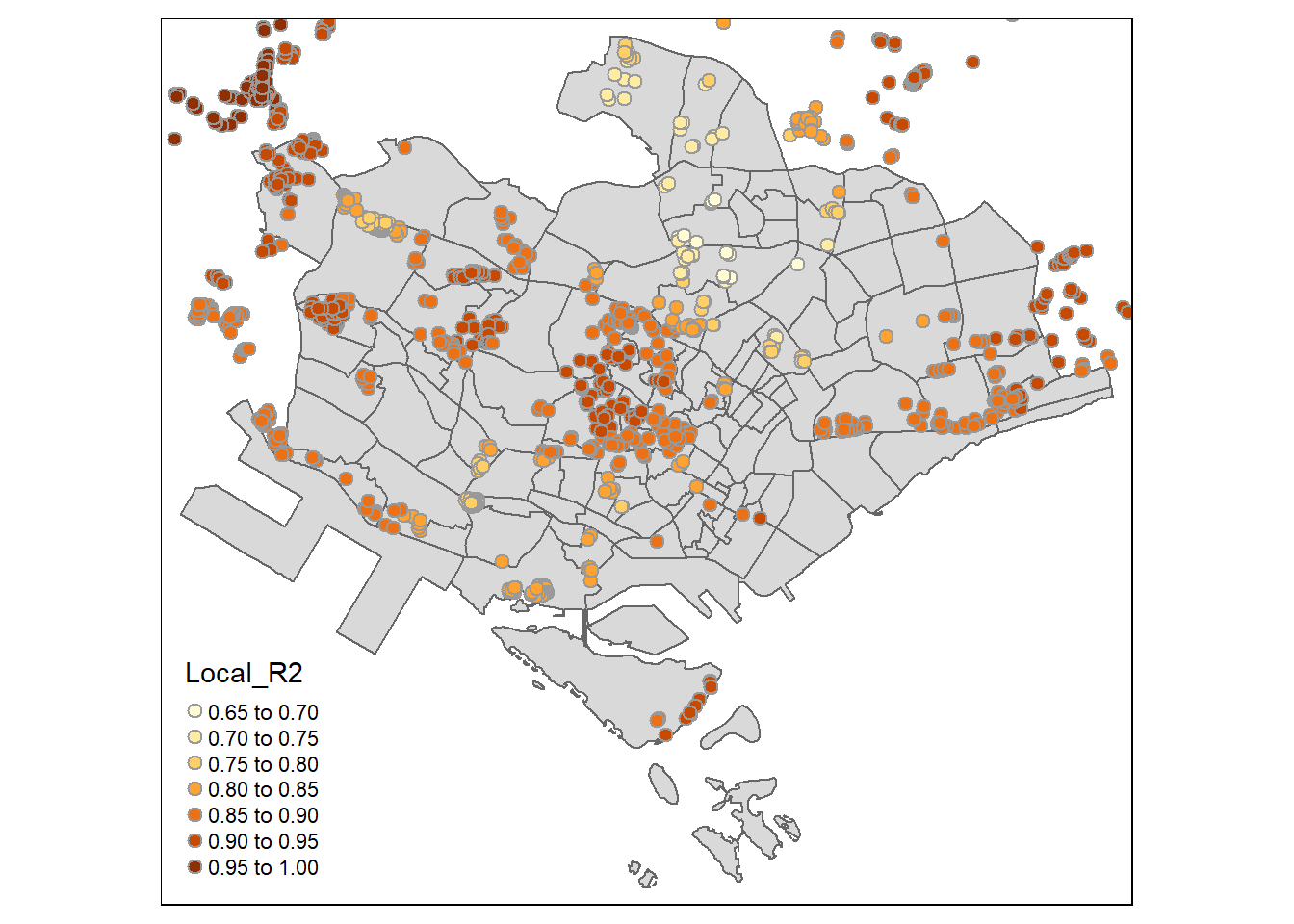
In the above map, we can see that the places which have darker static point symbols indicate that the local regression model fits well whereas very low values indicate the local model is performing poorly.
So, in this study, we have seen in detail how to build model with geographically weighted regression and the various steps in preparing the final data such as test for normality assumption, tests for non-linearity, checking multi collinearity. Some of the new concepts mentioned in this study are building publication table using Ordinary Least Square Regression OLSR) method and gtsummary method. Stay tuned for upcoming sections………………..