Loading packages
pacman::p_load(rgdal, spdep, tmap, sf,
               ggpubr, cluster, factoextra, NbClust,
heatmaply, corrplot, psych, tidyverse, purrr,ClustGeo)In today’s class exercise, lets see how to apply Spatially constrained clustering algorithm - ClustGeo Method to delineate homogeneous region of Vietnam.
Following two data sets are used:
Myanmar Township Boundary Data (i.e. myanmar_township_boundaries) : This is a GIS data in ESRI shapefile format. It consists of township boundary information of Myanmar. The spatial data are captured in polygon features.
Shan-ICT.csv: This is an extract of The 2014 Myanmar Population and Housing Census Myanmar at the township level.
p_load function pf pacman package is used to install and load sf all necessary packages into R environment.
sf, rgdal and spdep - Spatial data handling
tidyverse, especially readr, ggplot2 and dplyr - Attribute data handling
tmap -Choropleth mapping
coorplot, ggpubr, and heatmaply - Multivariate data visualisation and analysis
cluster, ClustGeo - Cluster analysis
The code chunk below installs and launches these R packages into R environment.
The Myanmar Township Boundary GIS data is in ESRI shapefile format. It is imported into R environment by using the st_read() function of sf. The imported InfoComm variables are extracted from The 2014 Myanmar Population and Housing Census Myanmar. The attribute data set is called ict. It is saved in R’s tibble data.frame format.
Reading layer `myanmar_township_boundaries' from data source
  `D:\raveenaclr\Geospatial Analytics\InClass_Ex\data3\geospatial'
  using driver `ESRI Shapefile'
Simple feature collection with 330 features and 14 fields
Geometry type: MULTIPOLYGON
Dimension:     XY
Bounding box:  xmin: 92.17275 ymin: 9.671252 xmax: 101.1699 ymax: 28.54554
Geodetic CRS: WGS 84It is wiser to take proportion of no. of households present instead of using the numbers directly. So, let us preprocess the data accordingly by using the code chunk below:
ict_derived <- ict %>%
  mutate(`RADIO_PR` = `Radio`/`Total households`*1000) %>%
  mutate(`TV_PR` = `Television`/`Total households`*1000) %>%
  mutate(`LLPHONE_PR` = `Land line phone`/`Total households`*1000) %>%
  mutate(`MPHONE_PR` = `Mobile phone`/`Total households`*1000) %>%
  mutate(`COMPUTER_PR` = `Computer`/`Total households`*1000) %>%
  mutate(`INTERNET_PR` = `Internet at home`/`Total households`*1000) %>%
  rename(`DT_PCODE` =`District Pcode`,`DT`=`District Name`,
         `TS_PCODE`=`Township Pcode`, `TS`=`Township Name`,
         `TT_HOUSEHOLDS`=`Total households`,
         `RADIO`=`Radio`, `TV`=`Television`,
         `LLPHONE`=`Land line phone`, `MPHONE`=`Mobile phone`,
`COMPUTER`=`Computer`, `INTERNET`=`Internet at home`) radio <- ggplot(data=ict_derived,
aes(x= `RADIO_PR`,
y= ..density..)) +
geom_histogram(bins=20,
color="black",
fill="coral")+
geom_density(color="black",
alpha = 0.2)
tv <- ggplot(data=ict_derived,
aes(x= `TV_PR`,
y= ..density..)) +
geom_histogram(bins=20,
color="black",
fill="coral")+
geom_density(color="red",
alpha = 0.2)
llphone <- ggplot(data=ict_derived,
aes(x= `LLPHONE_PR`,
y= ..density..)) +
geom_histogram(bins=20,
color="black",
fill="coral")+
geom_density(color="black",
alpha = 0.2)
mphone <- ggplot(data=ict_derived,
aes(x= `MPHONE_PR`,
y= ..density..)) +
geom_histogram(bins=20,
color="black",
fill="coral")+
geom_density(color="black",
alpha = 0.2)
computer <- ggplot(data=ict_derived,
aes(x= `COMPUTER_PR`,
y= ..density..)) +
geom_histogram(bins=20,
color="black",
fill="coral")+
geom_density(color="black",
alpha = 0.2)
internet <- ggplot(data=ict_derived,
aes(x= `INTERNET_PR`,
y= ..density..)) +
geom_histogram(bins=20,
color="black",
fill="coral")+
geom_density(color="black",
alpha = 0.)
ggarrange(radio, tv, llphone, mphone, computer, internet,
ncol = 3,
nrow = 2)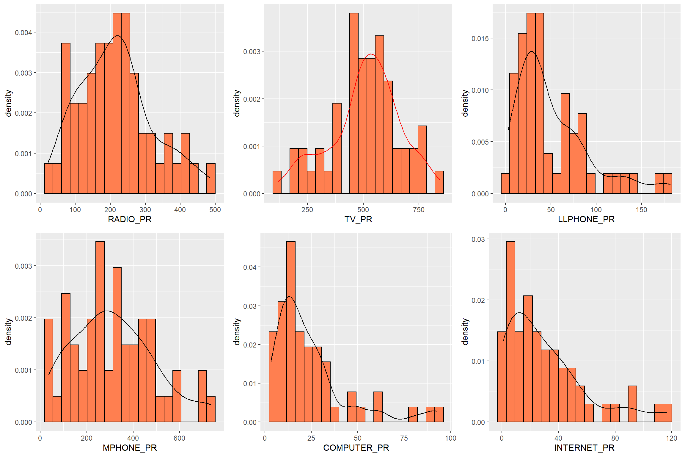
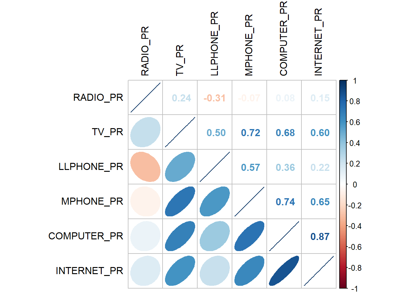
Before we perform cluster analysis, it is important for us to ensure that the cluster variables are not highly correlated.
In this section, you will learn how to use corrplot.mixed() function of corrplot package to visualise and analyse the correlation of the input variables.
Before we visualise the maps using choropleth, let us first combine both geospatial and aspatial datsets into one simple feature dataframe using the code chunk below.
Now let us perform hierarchical cluster analysis. The analysis consists of four major steps:
Extracting clustering variables
Data standardisation
Visualising the clustering variables
Computing Proximity Matrix
Extracting clustering variables
        TS.x RADIO_PR    TV_PR LLPHONE_PR MPHONE_PR COMPUTER_PR
1    Mongmit 286.1852 554.1313   35.30618  260.6944    12.15939
2    Pindaya 417.4647 505.1300   19.83584  162.3917    12.88190
3    Ywangan 484.5215 260.5734   11.93591  120.2856     4.41465
4   Pinlaung 231.6499 541.7189   28.54454  249.4903    13.76255
5     Mabein 449.4903 708.6423   72.75255  392.6089    16.45042
6      Kalaw 280.7624 611.6204   42.06478  408.7951    29.63160
7      Pekon 318.6118 535.8494   39.83270  214.8476    18.97032
8   Lawksawk 387.1017 630.0035   31.51366  320.5686    21.76677
9  Nawnghkio 349.3359 547.9456   38.44960  323.0201    15.76465
10   Kyaukme 210.9548 601.1773   39.58267  372.4930    30.94709
Now let us rename the township name instead of row number and delete the old one using the code chunk below
          RADIO_PR    TV_PR LLPHONE_PR MPHONE_PR COMPUTER_PR
Mongmit   286.1852 554.1313   35.30618  260.6944    12.15939
Pindaya   417.4647 505.1300   19.83584  162.3917    12.88190
Ywangan   484.5215 260.5734   11.93591  120.2856     4.41465
Pinlaung  231.6499 541.7189   28.54454  249.4903    13.76255
Mabein    449.4903 708.6423   72.75255  392.6089    16.45042
Kalaw     280.7624 611.6204   42.06478  408.7951    29.63160
Pekon     318.6118 535.8494   39.83270  214.8476    18.97032
Lawksawk  387.1017 630.0035   31.51366  320.5686    21.76677
Nawnghkio 349.3359 547.9456   38.44960  323.0201    15.76465
Kyaukme   210.9548 601.1773   39.58267  372.4930    30.94709
Data Standardisation
In order to avoid the cluster analysis result is baised to clustering variables with large values, it is useful to standardise the input variables before performing cluster analysis.
Performing Min-Max standardisation
In the code chunk below, normalize() of heatmaply package is used to stadardisation the clustering variables by using Min-Max method. The summary() is then used to display the summary statistics of the standardised clustering variables.
    RADIO_PR          TV_PR          LLPHONE_PR       MPHONE_PR
 Min.   :0.0000   Min.   :0.0000   Min.   :0.0000   Min.   :0.0000
 1st Qu.:0.2544   1st Qu.:0.4600   1st Qu.:0.1123   1st Qu.:0.2199
 Median :0.4097   Median :0.5523   Median :0.1948   Median :0.3846
 Mean   :0.4199   Mean   :0.5416   Mean   :0.2703   Mean   :0.3972
 3rd Qu.:0.5330   3rd Qu.:0.6750   3rd Qu.:0.3746   3rd Qu.:0.5608
 Max.   :1.0000   Max.   :1.0000   Max.   :1.0000   Max.   :1.0000
  COMPUTER_PR
 Min.   :0.00000
 1st Qu.:0.09598
 Median :0.17607
 Mean   :0.23692
 3rd Qu.:0.29868
 Max.   :1.00000
Performing Z-score standardisation
Z-score standardisation can be performed easily by using scale() of Base R. The code chunk below will be used to stadardisation the clustering variables by using Z-score method.
            vars  n mean sd median trimmed  mad   min  max range  skew kurtosis
RADIO_PR       1 55    0  1  -0.04   -0.06 0.94 -1.85 2.55  4.40  0.48    -0.27
TV_PR          2 55    0  1   0.05    0.04 0.78 -2.47 2.09  4.56 -0.38    -0.23
LLPHONE_PR     3 55    0  1  -0.33   -0.15 0.68 -1.19 3.20  4.39  1.37     1.49
MPHONE_PR      4 55    0  1  -0.05   -0.06 1.01 -1.58 2.40  3.98  0.48    -0.34
COMPUTER_PR    5 55    0  1  -0.26   -0.18 0.64 -1.03 3.31  4.34  1.80     2.96
              se
RADIO_PR    0.13
TV_PR       0.13
LLPHONE_PR  0.13
MPHONE_PR   0.13
COMPUTER_PR 0.13
We observe that mean and standard deviation of the Z-score standardised clustering variables are 0 and 1 respectively. We should take note that Z-score standardisation method should only be used if we would assume all variables come from some normal distribution.
Visualising the standardised clustering variables
Let us visualise the standardised clustering variables graphically in addition to summary statistics
r <- ggplot(data=ict_derived,
             aes(x= `RADIO_PR`)) +
  geom_histogram(bins=20,
                 color="black",
                 fill="light blue")+
  ggtitle("Before Standardisation")

shan_ict_s_df <- as.data.frame(shan_ict.std)
s <- ggplot(data=shan_ict_s_df,
       aes(x=`RADIO_PR`)) +
  geom_histogram(bins=20,
                 color="black",
                 fill="light blue") +
  ggtitle("Min-Max Standardisation")

shan_ict_z_df <- as.data.frame(shan_ict.z)
z <- ggplot(data=shan_ict_z_df,
       aes(x=`RADIO_PR`)) +
  geom_histogram(bins=20,
                 color="black",
                 fill="light blue") +
  ggtitle("Z-score Standardisation")

ggarrange(r, s, z,
          ncol = 3,
          nrow = 1)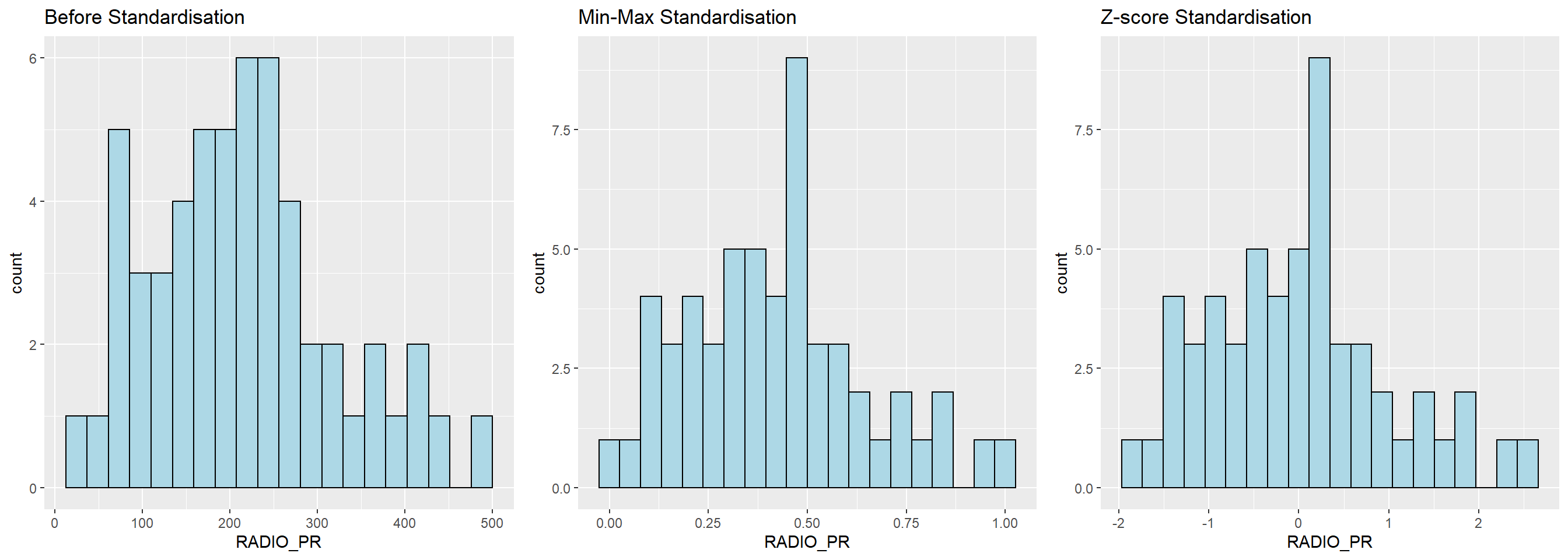
We can observe that after standardisation, the variables follow normal distribution.
Computing Proximity Matrix The code chunk below is used to compute the proximity matrix using euclidean method although the function dist() supports six distance proximity calculations, they are: euclidean, maximum, manhattan, canberra, binary and minkowski.
To perform non-spatially constrained hierarchical clustering, we only need to provide the function a dissimilarity matrix as shown in the code chunk below.
Similarly, we can plot the clusters on a categorical area shaded map by using the steps we learned in 5.7.12 Mapping the clusters formed.
Before we can performed spatially constrained hierarchical clustering, a spatial distance matrix will be derived by using st_distance() of sf package.
dist <- st_distance(shan_sf, shan_sf)
distmat <- as.dist(dist)
cr <- choicealpha(proxmat, distmat, range.alpha = seq(0, 1, 0.1), K=6, graph = TRUE)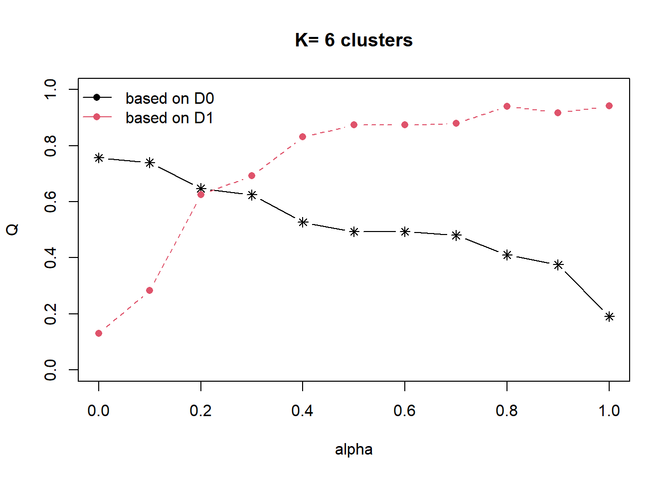
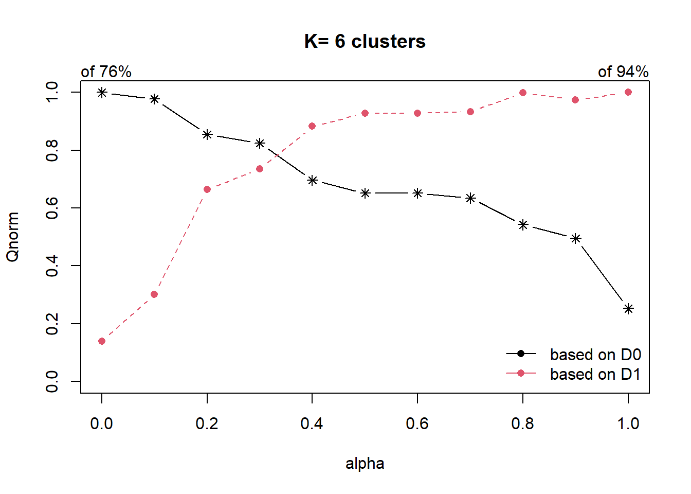
With reference to the graphs above, alpha = 0.3 will be used as shown in the code chunk below