Packages
pacman::p_load(sf, tidyverse, tmap, spdep, patchwork, ggthemes)For this study, data from WPdx Global Data Repositories and geoBoundaries are used. Both are in geospatial format. These dataset provide information about waterpoints and Nigeria’s Administrative boundary shape file.
| Data Type | Description | Source |
|---|---|---|
| Geospatial | Nigeria Level-2 Administrative Boundary | Geoboundaries |
| Geospatial | Water point related data on WPdx standard | Waterpoint access data |
Let us try to understand the dynamics of spatial patterns of non-functional water points in Nigeria and its diffusion over spatial boundaries using appropriate global and local measures of spatial association techniques.
Let us first load required packages into R environment. p_load function pf pacman package is used to install and load sf and tidyverse pacagkes into R environment.
Now let us import both the geospatial data. The code chunk below uses st_read() function of sf package to import geoBoundaries-NGA-ADM2_simplified shapefile and geo_export into R environment.
Two arguments are used :
dsn - destination : to define the data path
layer - to provide the shapefile name
st_read() of sf package is used to import geo_export and geoBoundaries-NGA-ADM2_simplified shapefile into R environment and save the imported geospatial data into simple feature data table.
filter() of dplyr package is used to extract water point records of Nigeria.
In order to reduce the file size let us save the data in .rds format.
write_rds() of readr package is used to save the extracted sf data table into an output file in rds data format.
Let us now preprocess the data before performing any analysis
Here, we are recoding the NA values into Unknown. In the code chunk below, replace_na() is used to recode all the NA values in status_cle field into Unknown.
As our objective is to focus on waterpoints, let us extract the three types and save it as a dataframe for further analysis
wpt_functional <- wp_nga %>%
  filter(status_cle %in%
           c("Functional",
             "Functional but not in use",
             "Functional but needs repair"))

wpt_nonfunctional <- wp_nga %>%
  filter(status_cle %in%
           c("Abandoned/Decommissioned",
             "Abandoned",
             "Non-Functional",
             "Non functional due to dry season",
             "Non-Functional due to dry season"))

wpt_unknown <- wp_nga %>%
  filter(status_cle == "Unknown")
In the code chunk above, filter() of dplyr is used to select the specific water points.
We have to perform 2 steps to calculate the total number of functional, non-functional and Unknown waterpoints in each division.
Let us identify no. of waterpoints located inside each division by using st_intersects().
Next, let us calculate numbers of pre-schools that fall inside each planning subzone by using length() function.
nga_wp <- nigeria %>%
  mutate(`total wpt` = lengths(
    st_intersects(nigeria, wp_nga))) %>%
  mutate(`wpt functional` = lengths(
    st_intersects(nigeria, wpt_functional))) %>%
  mutate(`wpt non-functional` = lengths(
    st_intersects(nigeria, wpt_nonfunctional))) %>%
  mutate(`wpt unknown` = lengths(
st_intersects(nigeria, wpt_unknown)))Now, let us calculate what is the overall proportion of functional and non-functional waterpoints by dividing the no. of functional waterpoints by the total no. of waterpoints. Similarly, for non-functional waterpoint proportion, numerator is replaced by non-functional waterpoint.
In order to manage the storage data efficiently, we are saving the final data frame in rds format.
Before performing spatial analysis, let us first do some preliminary data analysis to understand the data better in terms of water points.
Before visualising, its important for us to prepare the data. Based on WPDx Data Standard, the variable ‘#status_id’ refers to Presence of Water when Assessed. Binary response, i.e. Yes/No are recoded into Functional / Not-Functional.
ggplot(data= ngawater_sf,
       aes(x= `#status_id`)) +
       geom_bar(fill= '#CD5C5C') +
       #ylim(0, 150) +
       geom_text(stat = 'count',
           aes(label= paste0(stat(count), ', ',
                             round(stat(count)/sum(stat(count))*100,
                             1), '%')), vjust= -0.5, size= 2.5) +
       labs(y= 'No. of \nwater points',
            x= 'Water Points',
            title = "Distribution of water points") +
       theme(axis.title.y= element_text(angle=0),
             axis.ticks.x= element_blank(),
             panel.background= element_blank(),
             axis.line= element_line(color= 'grey'),
             axis.title.y.left = element_text(vjust = 0.5),
             plot.title = element_text(hjust=0.5))
Insights:
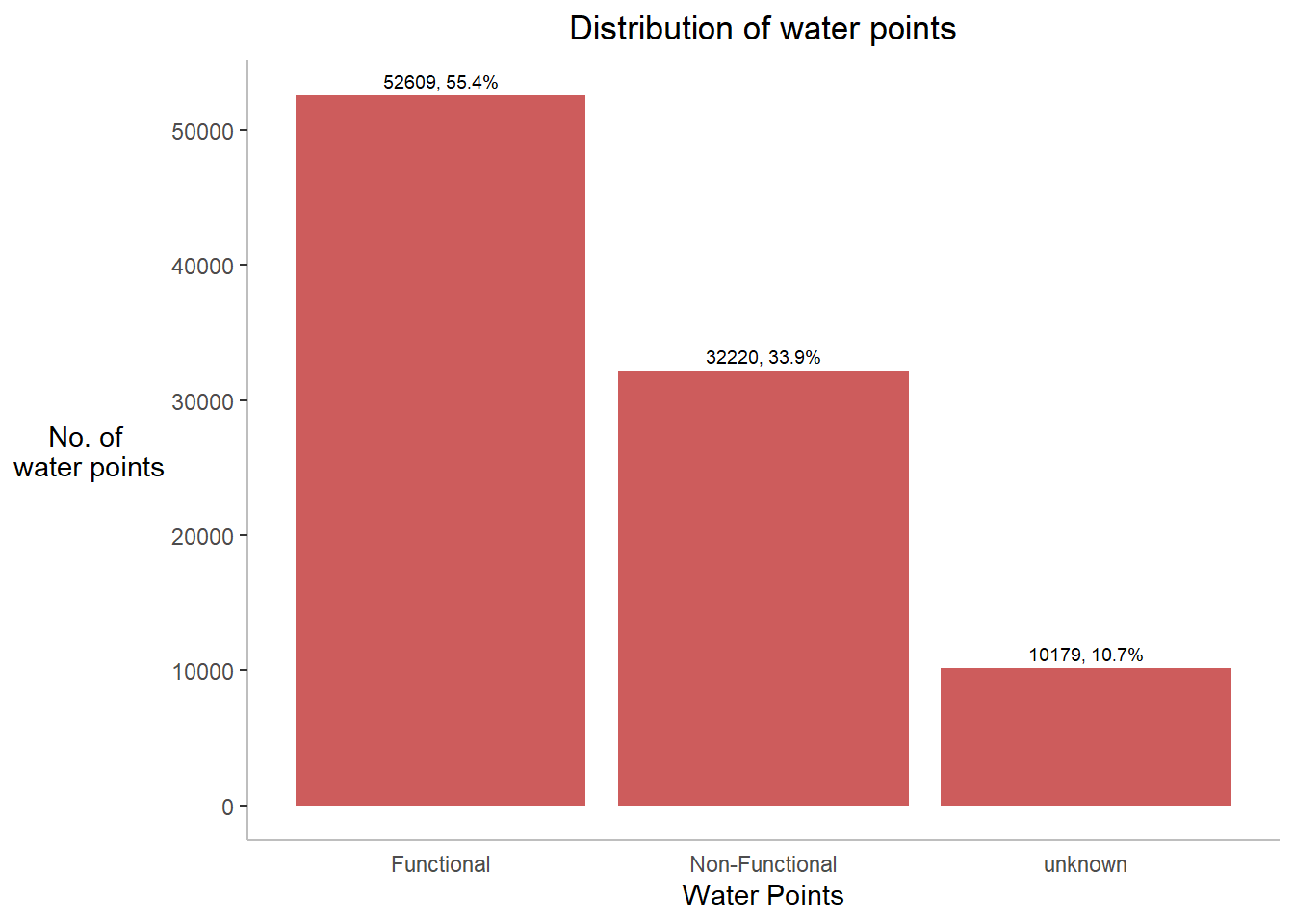
Nigeria consists of almost 55% of functional, 34% of non-functional and 11% of unknown waterpoints.
First let us prepare the data
p3 <- ggplot(data=top_10,
             aes(x=shapeName,
                 y=prop,
                 fill=waterpoint_status))+
  geom_col()+
  geom_text(aes(label=paste0(prop,"%")),
            position = position_stack(vjust=0.5),size=3)+
  theme(axis.text.x=element_text(angle=0))+
    xlab("Division")+
    ylab("% of \n Waterpoints")+
    ggtitle("Proportion of waterpoints by District")+
    theme_bw()+
    guides(fill=guide_legend(title="Waterpoint"),
           shape=guide_legend(override.aes = list(size=0.5)))+
    theme(plot.title = element_text(hjust=0.5, size=13),
          legend.title = element_text(size=9),
          legend.text = element_text(size=7),
          axis.text = element_text(face="bold"),
          axis.ticks.x=element_blank(),
          axis.title.y=element_text(angle=0),
          axis.title.y.left = element_text(vjust = 0.5))
p3
Insights:
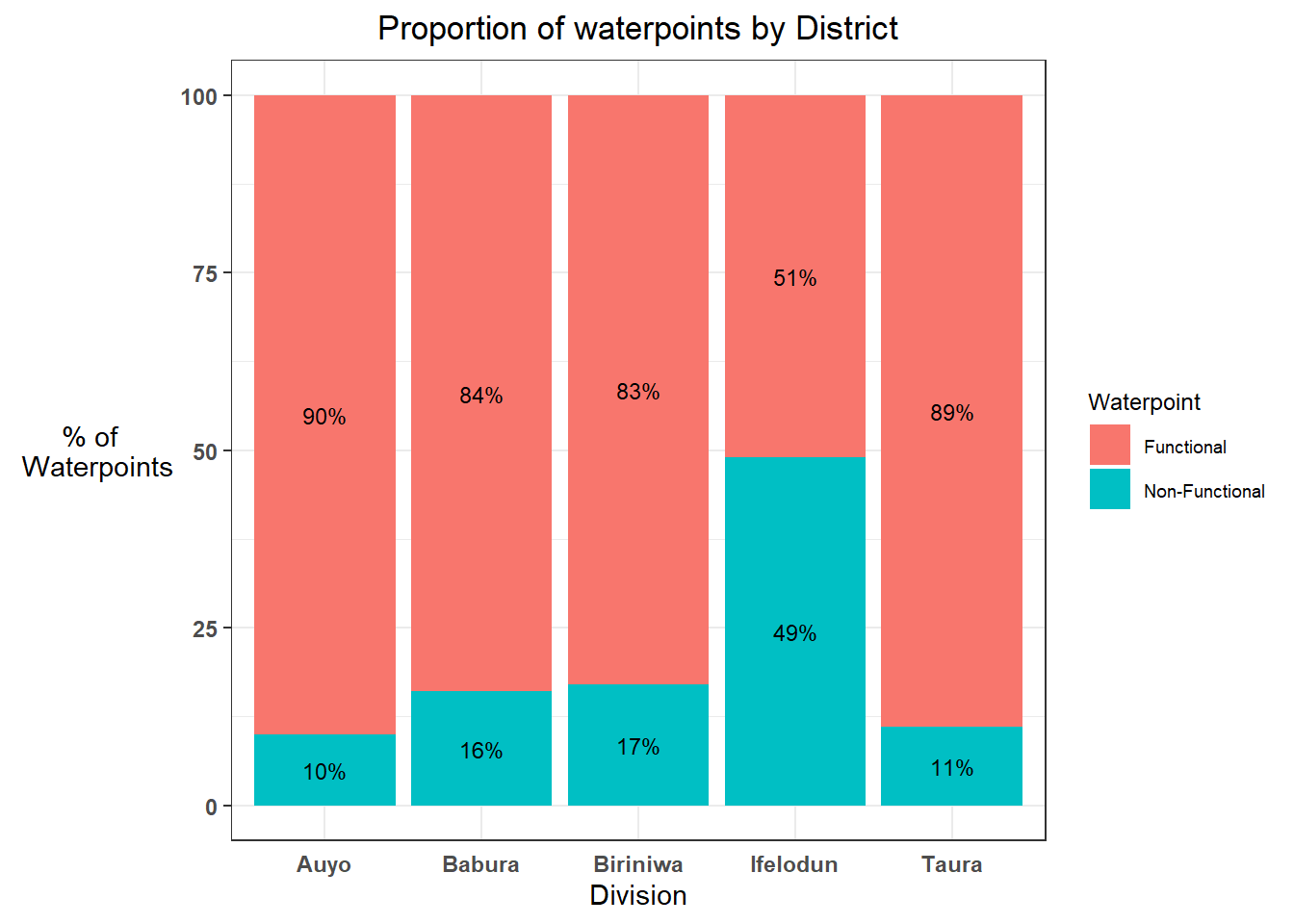
Among the divisions which have most no. of waterpoints, in Ifelodun division, almost 50% of waterpoints are non-functional. It is a matter of concern.
To find out the solution for this question, first let’s prepare the data accordingly:
ggplot(data = nonfunc_top10,
       aes(y = reorder(shapeName, n),
           x=n)) +
  geom_bar(stat = "identity",
           fill = "coral")+
  labs(y= 'Division',
       x='No. of Non-Functional water points',
       title="Top 10 divisions by Non-Functional waterpoints",) +
  geom_text(stat='identity', aes(label=paste0(n)),hjust=-0.5)+
  theme(axis.title.y=element_text(angle=0),
        axis.ticks.x=element_blank(),
        panel.background = element_blank(),
        axis.line = element_line(color='grey'),
        plot.title = element_text(hjust = 0.5),
        axis.title.y.left = element_text(vjust = 0.5),
        axis.text = element_text(face="bold") )
Insights:
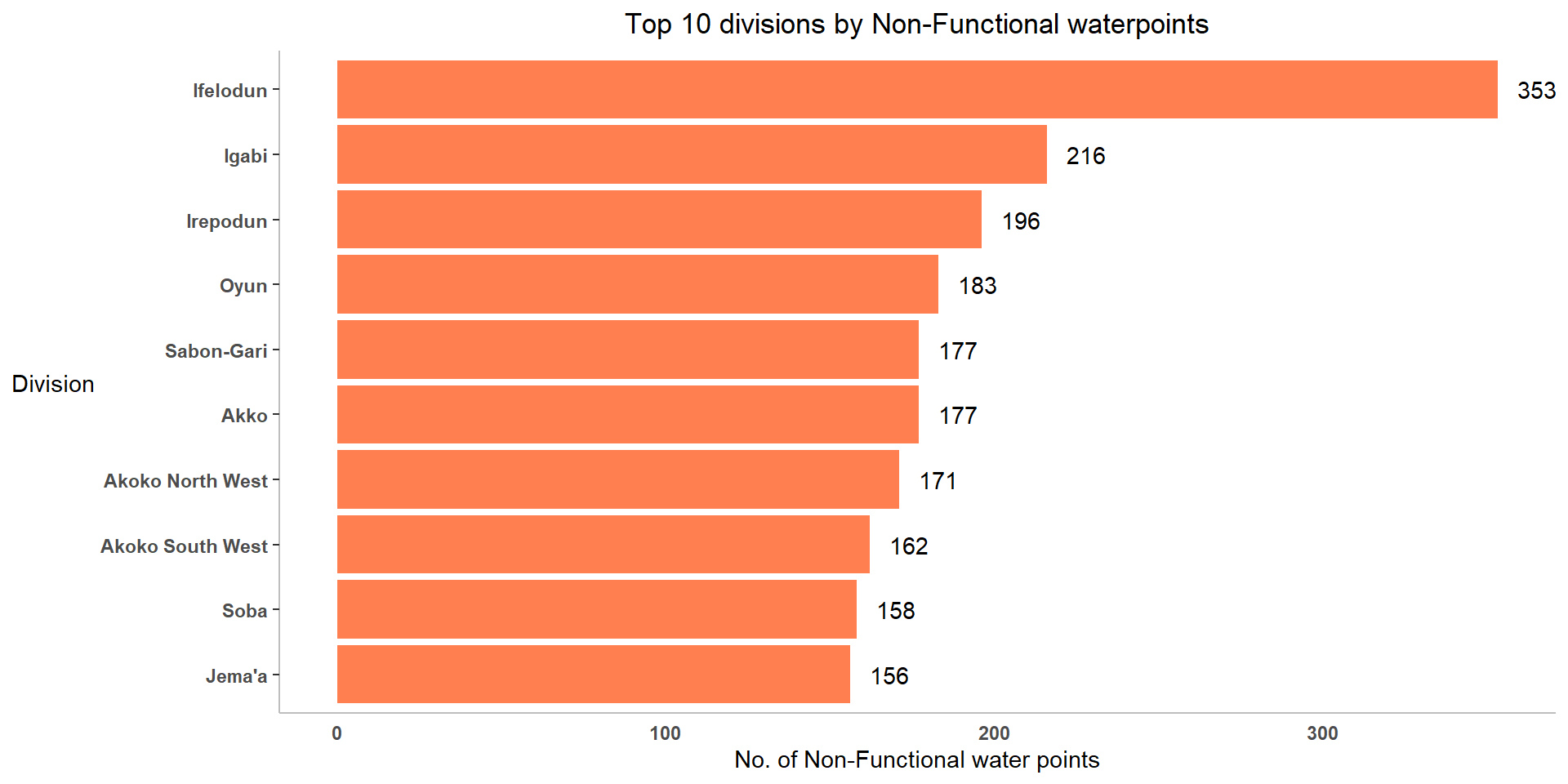
Among all 774 administrative level 2 divisions, Ifelodun has most no. of non-functional water points followed by Igabi, Irepodun, Oyun and Sabon-Gari.
As our objective is to focus more on non-functional waterpoints, let us try to understand what are the major causes for a water point to become non-functional and which contributes the most?
To find out the solution for this question, first let’s prepare the data accordingly:
wpt_nonfunctional <- read_rds("data2/wpt_nonfunctional.rds")
wpt_nonfunctional <- wpt_nonfunctional %>%
  mutate(status_cle=recode(status_cle,
                     'Non-Functional due to dry season'='Dry Season',
                     'Non functional due to dry season'='Dry Season',
                     'Abandoned/Decommissioned' = 'Abandoned / Decommissioned',
                     'Abandoned' = 'Abandoned / Decommissioned'))
nonfun_order <- factor(wpt_nonfunctional$status_cle, level = c('Non-Functional', 'Dry Season','Abandoned / Decommissioned'))ggplot(data= wpt_nonfunctional,
aes(x= nonfun_order)) +
geom_bar(fill= 'plum') +
#ylim(0, 150) +
geom_text(stat = 'count',
aes(label= paste0(stat(count), ', ',
round(stat(count)/sum(stat(count))*100,
1), '%')), vjust= -0.5, size= 2.5) +
labs(x= 'Reasons',
y= 'No. of \nwater points',
title = "What are the causes of non-functional water points?") +
theme(axis.title.y= element_text(angle=0),
axis.ticks.x= element_blank(),
panel.background= element_blank(),
axis.line= element_line(color= 'grey'),
axis.title.y.left = element_text(vjust = 0.5),
plot.title = element_text(hjust=0.5))
Insights:
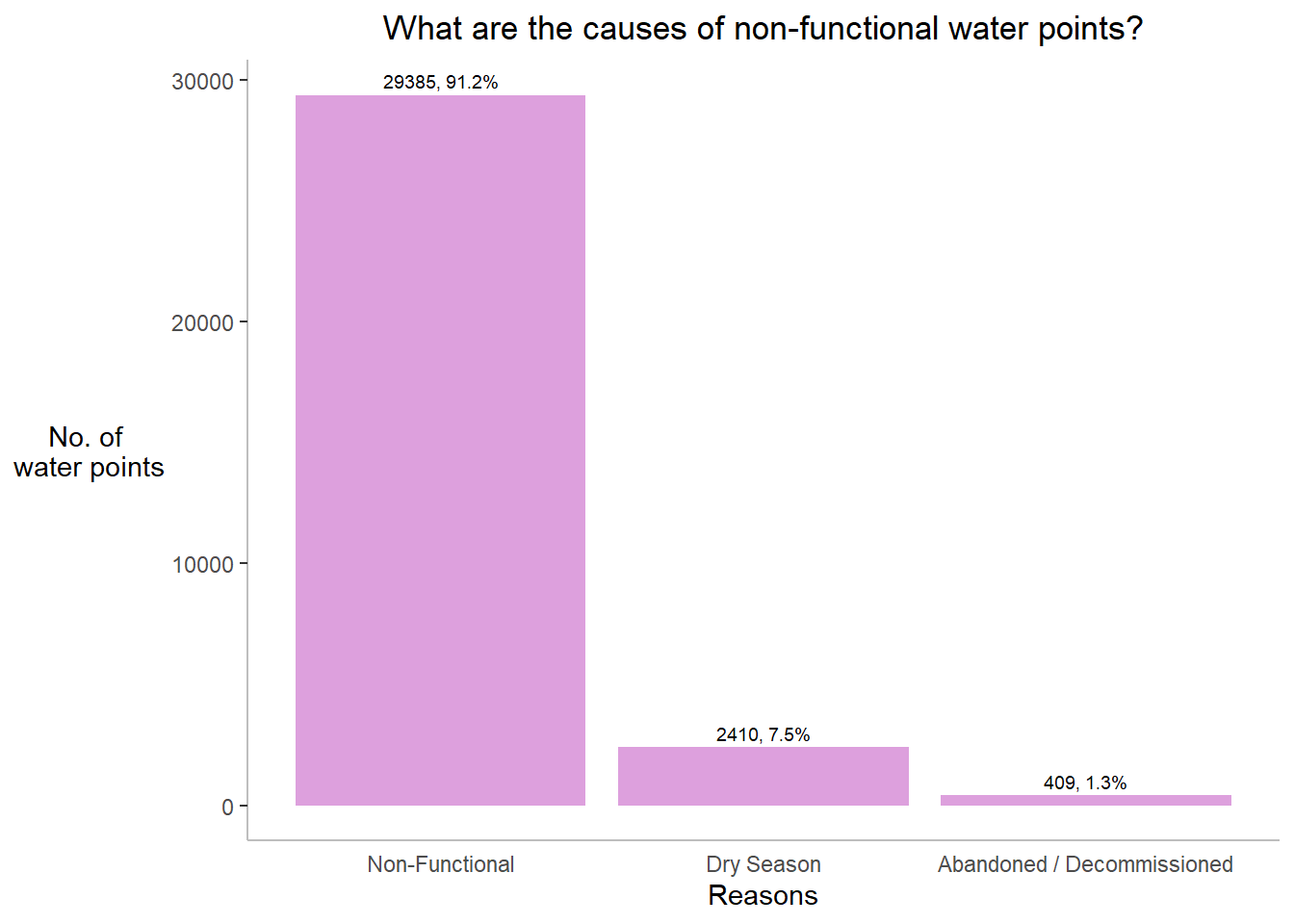
Almost 90% of non-functional waterpoints are not reason specific. Some other reasons include dry season , waterpoints are decommissioned or some are left without being taken care of.