REDCAP and AZP Spatial clustering

Spatial Clustering

Spatial clustering aims to group of a large number of geographic areas or points into a smaller number of regions based on similiarities in one or more variables. Spatially constrained clustering is needed when clusters are required to be spatially contiguous.

There are three different approaches explicitly incorporate the contiguity constraint in the optimization process:

SKATER
Redcap
AZP

rgeoda Package

rgeoda provides spatial data analysis functionalities including Exploratory Spatial Data Analysis, Spatial Cluster Detection and Clustering Analysis, Regionalization, etc.

Install Packages

Loading Packages

pacman::p_load(sf, tidyverse, tmap, rgeoda,
               plotly, GGally, spdep)

Reading Data files

nga_derived <- read_rds("data/nga_derived.rds")
nga_wp_clus <- read_rds("data/nga_wp_clus.rds")

1. REDCAP

REDCAP (Regionalization with dynamically constrained agglomerative clustering and partitioning) is developed by D. Guo (2008). Like SKATER, REDCAP starts from building a spanning tree in 3 different ways (single-linkage, average-linkage, and the complete-linkage). The single-linkage way leads to build a minimum spanning tree. Then, REDCAP provides 2 different ways (first-order and full-order constraining) to prune the tree to find clusters. The first-order approach with a minimum spanning tree is the same as SKATER. In GeoDa and rgeoda, the following methods are provided:

First-order and Single-linkage
Full-order and Complete-linkage
Full-order and Average-linkage
Full-order and Single-linkage
Full-order and Wards-linkage

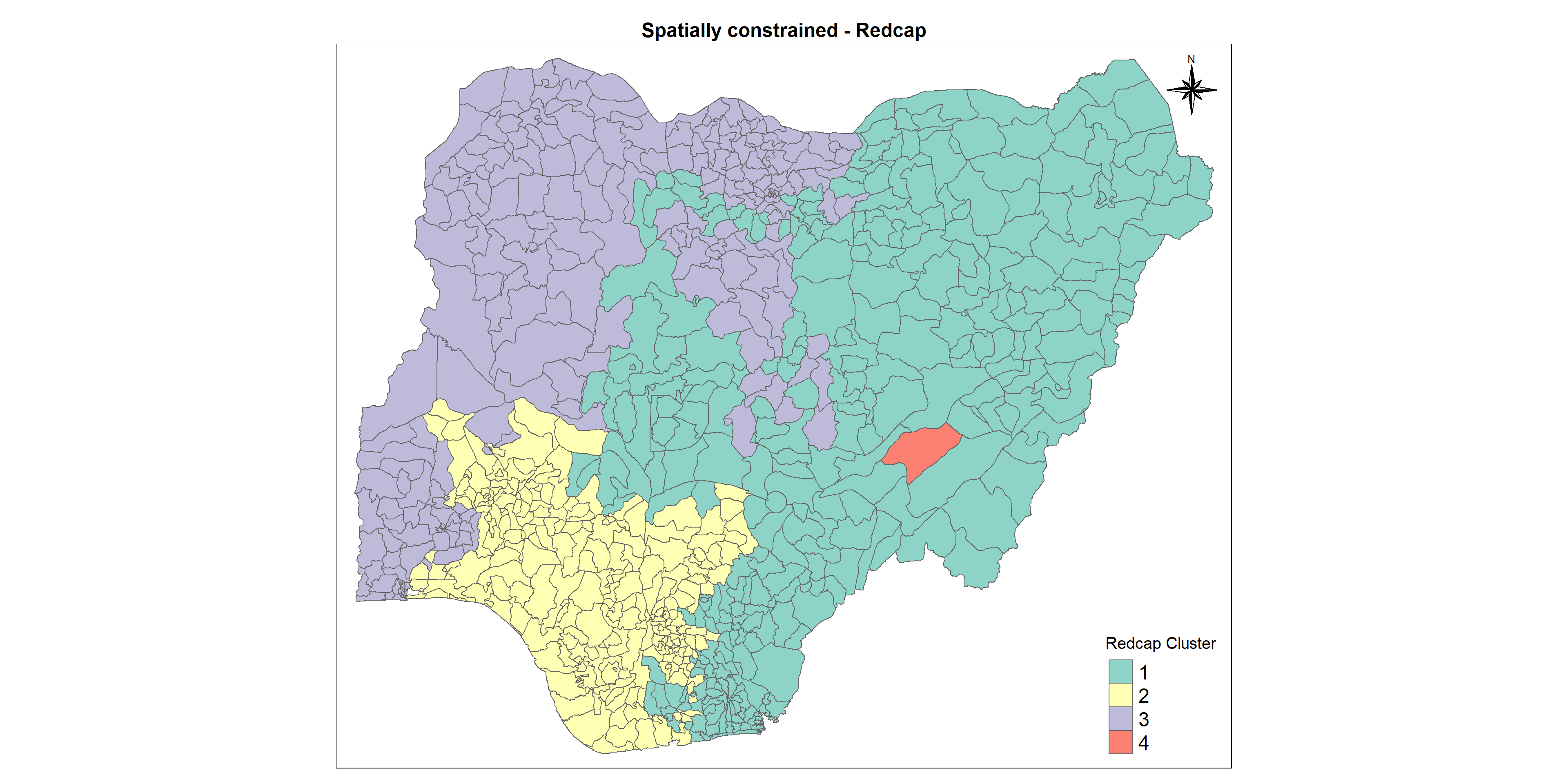
For example, to find 4 clusters using the same dataset and weights as above using REDCAP with Full-order and Complete-linkage method

We have to remove the region which has no neighbours while creating a Queen contiguity weight

nga_wp_clusf = nga_wp_clus %>%
                       filter(shapeName != "Bakassi")

queen_w <- queen_weights(nga_wp_clusf)

The below code chunk is to compute REDCAP clusters with fullorder complete linkage method using redcap() of rgeoda package.

redcap_clusters <- redcap(k = 4, 
                          w = queen_w, 
                          df = nga_derived, 
                          method = "fullorder-completelinkage")

The code chunk below form the join in three steps:

the redcap_clusters list object will be converted into a matrix;
cbind() is used to append groups matrix onto nga_wp_clusf to produce an output simple feature object called redcapClusterand
rename of dplyr package is used to rename as.matrix.groups field as Redcap_Cluster

redcap_cluster <- as.matrix(redcap_clusters$Clusters)
redcapCluster <- cbind(nga_wp_clusf, as.factor(redcap_cluster)) %>%
  rename(`Redcap_Cluster`=`as.factor.redcap_cluster.`)

Let us map the clusters and view its spatial distribution using tmap options

cmap1 <- tm_shape (redcapCluster) +
          tm_polygons("Redcap_Cluster",
          title = "Redcap Cluster") +
          tm_layout(main.title = "Spatially constrained - Redcap",
                    main.title.position = "center",
                    main.title.size = 1.5,
                    legend.height = 1.5, 
                    legend.width = 1.5,
                    legend.text.size = 1.5,
                    legend.title.size = 1.5,
                    main.title.fontface = "bold",
                    frame = TRUE) +
        tmap_mode("plot")+
        tm_borders(alpha = 0.5) +
        tm_compass(type="8star",
                  position=c("right", "top"))

tmap mode set to plotting

cmap1

Warning: One tm layer group has duplicated layer types, which are omitted. To
draw multiple layers of the same type, use multiple layer groups (i.e. specify
tm_shape prior to each of them).

Visual interpretation of clusters - Parallel Plot

To reveal the clustering variables by cluster very effectively, let us create parallel coordinate plot using the code chunk below, ggparcoord() of GGally package

REDCAP - Parallel plot

p <- ggparcoord(data = redcapCluster,
           columns = c(7,8,16,17,18,20:23),
           scale = "std",
           alphaLines = 0.2,
           boxplot = TRUE,
           groupColumn = "Redcap_Cluster",
           title = "Multiple Parallel Coordinates Plots of REDCAP Cluster") +
  theme_minimal()+
  scale_color_manual(values=c( "#69b3a2", "red", "blue", "green") )+
  facet_grid(~ `Redcap_Cluster`) +
  theme(axis.text.x = element_text(angle = 30,size = 5))+
  xlab("")

ggplotly(p)

Interpretation:

It is alarming that in cluster 2 no. of non-functional points is greater than no. of functional points. Also most of the waterpoints here are in urban regions. The cruciality of waterpoints is the same for all the clusters whereas the waterpoints with higher score of staleness (the fact of not being fresh and tasting or smelling unpleasant) are more in cluster 1 and cluster 2 which are to be taken care of.

2. SKATER

The Spatial C(K)luster Analysis by Tree Edge Removal(SKATER) algorithm introduced by Assuncao et al. (2006) is based on the optimal pruning of a minimum spanning tree that reflects the contiguity structure among the observations. It provides an optimized algorithm to prune to tree into several clusters that their values of selected variables are as similar as possible.

The code chunk below computes SKATER clusters using skater() function of rgeoda package

SKATER_clusters <- rgeoda::skater(k = 4, 
                          w = queen_w, 
                          df = nga_derived )

aaa0after gda_skater

The code chunk below form the join in three steps:

the SKATER_clusters list object will be converted into a matrix;
cbind() is used to append groups matrix onto nga_wp_clusf to produce an output simple feature object called skaterCluster
rename of dplyr package is used to rename as.matrix.groups field as SKATER_Cluster

SKATER_cluster <- as.matrix(SKATER_clusters$Clusters)
skaterCluster <- cbind(nga_wp_clusf, as.factor(SKATER_cluster)) %>%
  rename(`SKATER_Cluster`=`as.factor.SKATER_cluster.`)

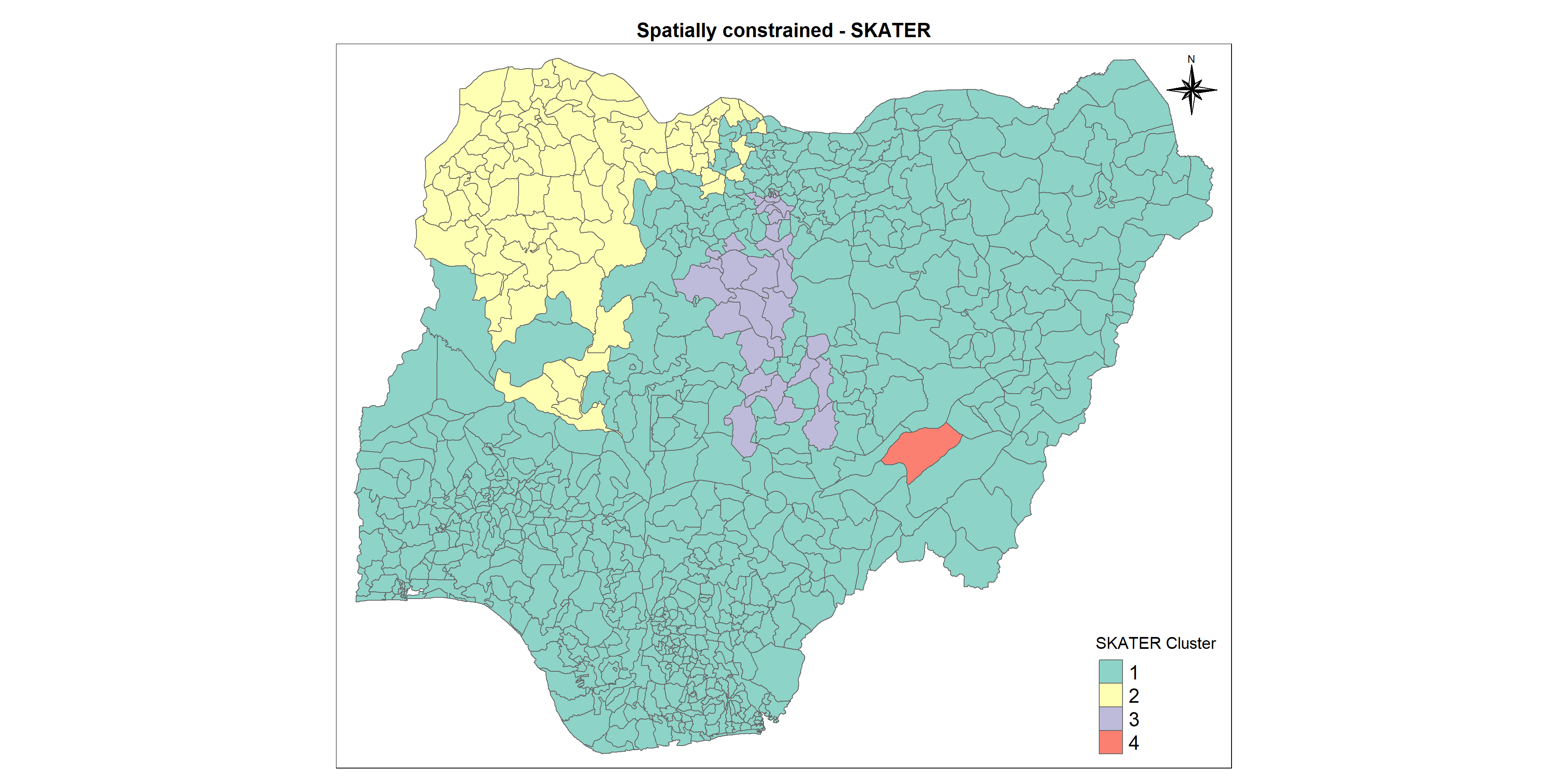
Let us map the clusters and view its spatial distribution using tmap options

cmap2 <- tm_shape (skaterCluster) +
          tm_polygons("SKATER_Cluster",
          title = "SKATER Cluster") +
          tm_layout(main.title = "Spatially constrained - SKATER",
                    main.title.position = "center",
                    main.title.size = 1.5,
                    legend.height = 1.5, 
                    legend.width = 1.5,
                    legend.text.size = 1.5,
                    legend.title.size = 1.5,
                    main.title.fontface = "bold",
                    frame = TRUE) +
        tmap_mode("plot")+
        tm_borders(alpha = 0.5) +
        tm_compass(type="8star",
                  position=c("right", "top"))

tmap mode set to plotting

cmap2

Warning: One tm layer group has duplicated layer types, which are omitted. To
draw multiple layers of the same type, use multiple layer groups (i.e. specify
tm_shape prior to each of them).

Visual interpretation of clusters - Parallel Plot

To reveal the clustering variables by cluster very effectively, let us create parallel coordinate plot using the code chunk below, ggparcoord() of GGally package

SKATER - Parallel plot

p <- ggparcoord(data = skaterCluster,
           columns = c(7,8,16,17,18,20:23),
           scale = "std",
           alphaLines = 0.2,
           boxplot = TRUE,
           groupColumn = "SKATER_Cluster",
           title = "Multiple Parallel Coordinates Plots of SKATER Cluster") +
  theme_minimal()+
  scale_color_manual(values=c( "#69b3a2", "red", "blue", "green") )+
  facet_grid(~ `SKATER_Cluster`) +
  theme(axis.text.x = element_text(angle = 30, size = 5))+
  xlab("")

ggplotly(p)

Interpretation:

Proportion of functional waterpoints is greater than non functional waterpoints in both clusters 1 and 2 which is very good sign and also the percentage of waterpoints with high staleness is lesser in numbers in cluster 2 which is again positive. But the same staleness percentage is quite high in cluster 1 which is a matter of concern.

3. AZP

The automatic zoning procedure (AZP) was initially outlined in Openshaw (1977) as a way to address some of the consequences of the modifiable areal unit problem (MAUP). In essence, it consists of a heuristic to find the best set of combinations of contiguous spatial units into p regions, minimizing the within-sum of squares as a criterion of homogeneity. The number of regions needs to be specified beforehand, as in most other clustering methods considered so far.

rgeoda provides three different heuristic algorithms to find an optimal solution for AZP:

greedy
Tabu Search
Simulated Annealing

a) AZP Greedy

The original AZP heuristic is a local optimization procedure that cycles through a series of possible swaps between spatial units at the boundary of a set of regions. The process starts with an initial feasible solution, i.e., a grouping of n spatial units into p contiguous regions. This initial solution can be constructed in several different ways. The initial solution must satisfy the contiguity constraints. For example, this can be accomplished by growing a set of contiguous regions from p randomly selected seed units by adding neighboring locations until the contiguity constraint can no longer be met.

azp_greedyclusters <- azp_greedy(p = 4, 
                           w = queen_w, 
                           df = nga_derived)

b) AZP Tabu Search

To use tabu search algorithm in maxp function, we can specify the parameters of tabu_length and conv_tabu:

azp_tabuclusters <- azp_tabu(p = 4, 
                         w = queen_w, 
                         df = nga_derived, 
                         tabu_length = 10, 
                         conv_tabu = 10)

c) AZP Simulated Annealing

To apply simulated annealing algorithm in maxp function with the parameter of cooling rate:

azp_clusters <- azp_sa( p = 4, 
                        w = queen_w, 
                        df = nga_derived, 
                        cooling_rate = 0.85)
azp_clusters

$Clusters
  [1] 1 1 1 3 2 1 2 2 1 1 1 2 2 2 2 1 2 1 1 3 1 2 1 3 1 1 1 2 2 1 1 2 1 2 2 1 2
 [38] 2 1 1 2 2 1 1 1 1 1 3 2 1 1 1 1 1 1 1 1 1 3 1 1 2 1 3 3 1 1 2 1 1 2 2 1 3
 [75] 2 2 1 1 1 1 1 1 1 3 1 3 3 2 1 1 2 1 2 1 3 3 2 1 2 3 1 2 1 1 2 1 1 3 2 1 3
[112] 3 3 2 3 2 2 1 1 1 1 1 2 2 1 1 3 3 2 3 2 2 1 1 2 2 2 3 2 3 3 2 1 1 1 3 3 3
[149] 3 3 1 1 3 2 1 1 1 1 1 2 1 1 2 1 2 3 3 2 1 1 2 1 1 1 1 2 2 2 1 1 1 1 1 1 1
[186] 1 1 1 1 2 1 1 1 1 1 1 1 2 1 1 1 1 1 1 1 1 2 1 1 2 1 2 2 2 1 1 1 3 3 3 2 1
[223] 2 1 3 2 3 2 1 1 1 2 1 3 1 1 1 3 2 1 3 1 1 3 1 1 2 3 2 3 2 1 1 1 3 2 1 3 1
[260] 1 3 2 3 3 2 4 2 1 1 1 2 2 1 1 2 2 2 2 2 1 2 2 1 2 1 1 2 2 2 2 1 2 2 1 2 1
[297] 2 1 1 1 1 1 1 1 1 2 2 1 1 1 1 1 1 1 2 2 2 2 1 1 1 1 3 1 1 2 2 2 1 1 1 2 1
[334] 1 1 1 1 1 1 1 1 1 2 3 2 1 2 1 3 2 1 2 1 2 1 2 1 3 2 2 2 2 1 1 1 1 1 1 2 1
[371] 1 1 1 2 1 1 2 2 1 1 1 1 1 1 3 2 2 3 2 1 1 1 4 2 3 3 2 3 1 2 1 3 2 2 1 3 2
[408] 1 3 2 1 2 2 3 2 1 1 3 3 2 1 1 3 2 1 2 3 2 1 1 2 1 3 2 3 3 2 1 1 1 1 2 2 3
[445] 3 1 2 1 2 3 1 1 2 1 1 3 2 1 1 2 2 2 1 1 3 2 1 2 1 2 1 1 3 2 3 2 3 2 1 1 3
[482] 3 2 2 3 2 1 3 3 2 1 3 1 3 3 2 2 2 1 1 1 3 1 1 2 1 2 1 2 2 1 1 3 2 2 1 1 2
[519] 1 1 1 1 1 1 2 3 2 2 2 1 1 1 1 1 2 2 1 1 1 2 1 1 2 2 1 1 1 1 1 1 1 2 1 1 2
[556] 2 1 2 2 1 2 1 2 1 1 2 2 2 1 1 1 2 1 1 1 1 1 1 1 2 2 1 1 2 1 1 1 1 1 1 2 1
[593] 1 2 2 1 1 2 1 1 1 1 2 1 1 1 2 1 2 1 1 2 1 1 1 1 1 1 1 1 1 2 2 1 1 1 1 1 1
[630] 1 2 1 2 1 1 2 2 2 2 3 2 1 2 1 1 2 3 3 2 1 3 3 3 2 1 3 1 2 3 3 3 2 3 2 1 3
[667] 2 1 1 1 3 3 2 1 1 1 3 2 2 1 2 3 2 3 3 2 1 1 1 1 3 2 2 1 1 1 1 1 3 3 3 2 2
[704] 2 1 3 1 2 1 3 1 2 3 2 1 1 2 2 1 1 1 1 1 1 2 1 1 2 1 3 1 2 1 1 1 1 2 2 1 3
[741] 2 2 2 1 1 1 3 2 1 1 3 3 3 2 1 1 1 1 1 3 2 1 1 1 1 1 1 1 2 3 1 3 3

$`Total sum of squares`
[1] 6957

$`Within-cluster sum of squares`
[1] 747.3657 700.0637 635.9083 519.1652 666.1842 596.0765 526.5721 582.3839
[9] 762.0337

$`Total within-cluster sum of squares`
[1] 1221.247

$`The ratio of between to total sum of squares`
[1] 0.1755421

Let us perform the join as we did in previous methods. The code chunk below form the join in three steps:

the azp_clusters list object will be converted into a matrix;
cbind() is used to append groups matrix onto nga_wp_clusf to produce an output simple feature object called AZPCluster
rename of dplyr package is used to rename as.factor.azp_cluster..groups field as AZP_Cluster

azp_cluster <- as.matrix(azp_clusters$Clusters)
AZPCluster <- cbind(nga_wp_clusf, as.factor(azp_cluster)) %>%
  rename(`AZP_Cluster`=`as.factor.azp_cluster.`)

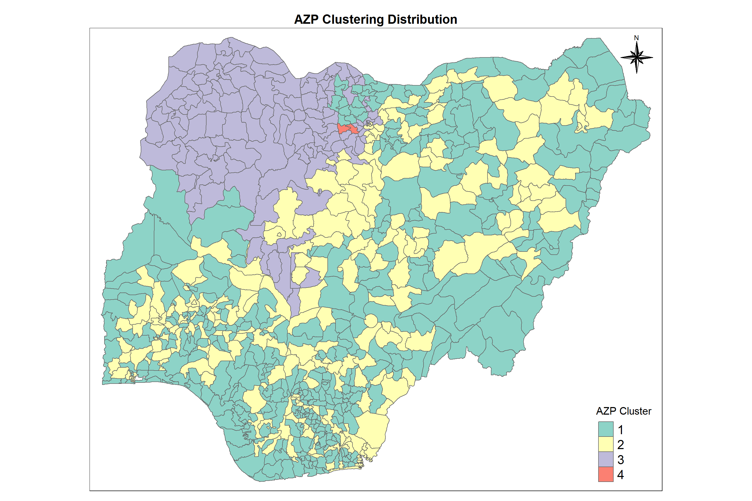
Let us map the clusters and view its spatial distribution using tmap options

cmap3 <- tm_shape (AZPCluster) +
          tm_polygons("AZP_Cluster",
          title = "AZP Cluster") +
          tm_layout(main.title = "AZP Clustering Distribution",
                    main.title.position = "center",
                    main.title.size = 1.5,
                    legend.height = 1.5, 
                    legend.width = 1.5,
                    legend.text.size = 1.5,
                    legend.title.size = 1.5,
                    main.title.fontface = "bold",
                    frame = TRUE) +
        tmap_mode("plot")+
        tm_borders(alpha = 0.5) +
        tm_compass(type="8star",
                  position=c("right", "top"))

tmap mode set to plotting

cmap3

Visual interpretation of clusters - Parallel Plot

AZP - Parallel plot

p <- ggparcoord(data = AZPCluster,
           columns = c(7,8,16,17,18,20:23),
           scale = "std",
           alphaLines = 0.2,
           boxplot = TRUE,
           groupColumn = "AZP_Cluster",
           title = "Multiple Parallel Coordinates Plots of AZP Cluster") +
  theme_minimal()+
  scale_color_manual(values=c( "#69b3a2", "red", "blue", "green") )+
  facet_grid(~ `AZP_Cluster`) +
  theme(axis.text.x = element_text(angle = 30, size=5))+
  xlab("")

ggplotly(p)

Interpretation:

We can infer from the chart that we are substantiating the results of REDCAP where in cluster 2 no. of non-functional points is greater than no. of functional points. Also most of the waterpoints here are in urban regions. The cruciality of waterpoints is the same for all the clusters whereas the waterpoints with higher score of staleness (the fact of not being fresh and tasting or smelling unpleasant) are more in cluster 1 and cluster 2 which are to be taken care of.

tmap_arrange(cmap1, cmap2, cmap3,
             ncol = 3)